Regression and adjusted comparisonsการวิเคราะห์ถดถอยและการเปรียบเทียบหลังปรับตัวแปรกวน
Logistic and linear regression with adjusted comparisons, and an add-on model comparisonการวิเคราะห์ถดถอยโลจิสติกและถดถอยเชิงเส้น การเปรียบเทียบที่ปรับอิทธิพลของตัวแปรกวน และการเปรียบเทียบแบบจำลองเมื่อเพิ่มตัวบ่งชี้ใหม่
An invented community health programme for older adults lent each of 420 participants, aged 60 to 79 years, a wrist activity tracker for 7 days at enrolment and took their average daily steps as the exposure of interest. At enrolment it also recorded age, sex, body-mass index, self-rated health, knee or hip pain, a six-minute walk distance and a timed up-and-go test. Everyone was followed for 12 months: 102 participants (24.3%) reported at least one fall (the binary outcome), and everyone repeated the six-minute walk at the end (the continuous outcome). The study is observational: nobody was asked to change how much they walk. The programme, the participants and every value are invented: all data are simulated with a fixed seed.โครงการสุขภาพชุมชนสมมุติสำหรับผู้สูงอายุแห่งหนึ่งให้ผู้เข้าร่วม 420 คน อายุ 60 ถึง 79 ปี ยืมสายรัดข้อมือวัดกิจกรรม (activity tracker) ไปสวม 7 วันตอนลงทะเบียน และใช้จำนวนก้าวเฉลี่ยต่อวันเป็นปัจจัยที่สนใจ (exposure) ตอนลงทะเบียนยังบันทึกอายุ เพศ ดัชนีมวลกาย ภาวะสุขภาพที่ประเมินด้วยตนเอง อาการปวดเข่าหรือสะโพก ระยะทางการเดินในหกนาที (six-minute walk distance) และผลการทดสอบ Timed Up and Go (TUG) ผู้เข้าร่วมทุกคนได้รับการติดตาม 12 เดือน มี 102 คน (24.3%) ที่รายงานว่าหกล้มอย่างน้อยหนึ่งครั้ง (ผลลัพธ์แบบสองค่า) และทุกคนทดสอบเดินหกนาทีซ้ำเมื่อสิ้นสุดการติดตาม (ผลลัพธ์แบบต่อเนื่อง) การศึกษานี้เป็นการศึกษาเชิงสังเกต (observational study) ไม่ได้กำหนดให้ผู้ใดเปลี่ยนปริมาณการเดิน โครงการ ผู้เข้าร่วม และค่าทุกค่าเป็นเรื่องสมมุติ ข้อมูลทั้งหมดเป็นข้อมูลจำลองที่สร้างด้วย seed คงที่
What you receiveสิ่งที่คุณจะได้รับ
Logistic or linear regression for a binary or continuous outcome: crude and adjusted estimates, and a comparison of models with and without an added predictor.วิเคราะห์ถดถอยโลจิสติกหรือถดถอยเชิงเส้น สำหรับผลลัพธ์แบบสองค่าหรือแบบต่อเนื่อง ได้ทั้งค่าประมาณก่อนและหลังปรับตัวแปรกวน และการเปรียบเทียบแบบจำลองเมื่อเพิ่มตัวแปรทำนายเข้าไป
- Crude and adjusted estimates (odds ratios or mean differences), each with a 95% confidence interval.ค่าประมาณก่อนและหลังปรับ (odds ratio หรือผลต่างค่าเฉลี่ย) พร้อมช่วงความเชื่อมั่น 95%
- A record of how the adjustment variables were chosen and how the model assumptions were checked.บันทึกเหตุผลในการเลือกตัวแปรที่ใช้ปรับ และผลการตรวจข้อตกลงเบื้องต้นของแบบจำลอง
- An add-on comparison showing what a new predictor adds to an existing model.การเปรียบเทียบแบบจำลองว่าตัวแปรทำนายใหม่ช่วยให้แบบจำลองเดิมดีขึ้นเพียงใด
- Result tables and an adjusted-effect plot.ตารางผลการวิเคราะห์ และกราฟแสดงขนาดผลหลังปรับ
The sampleตัวอย่างงาน
Sample work on simulated data. No real patient, no client project.ตัวอย่างงานจากข้อมูลจำลองทั้งหมด ไม่ใช่ข้อมูลผู้ป่วยจริง และไม่ใช่งานของลูกค้ารายใด
What this sample containsสิ่งที่อยู่ในตัวอย่างนี้
- Table 1: logistic regression, crude and adjusted odds ratios with 95% CI and P values.ตารางที่ 1 การวิเคราะห์ถดถอยโลจิสติก (logistic regression) แสดง odds ratio แบบหยาบและแบบปรับ พร้อม 95% CI และค่า P
- Table 2: linear regression, crude and adjusted coefficients with 95% CI.ตารางที่ 2 การวิเคราะห์ถดถอยเชิงเส้น (linear regression) แสดงสัมประสิทธิ์แบบหยาบและแบบปรับ พร้อม 95% CI
- Figure 1: the adjusted predicted probability of the outcome across the exposure, with its 95% CI.รูปที่ 1 ความน่าจะเป็นของผลลัพธ์ที่ทำนายจากแบบจำลองที่ปรับแล้วตามระดับของปัจจัยที่สนใจ พร้อม 95% CI
- Table 3: does a new marker add information? Likelihood-ratio test, AIC, and AUC with the DeLong test.ตารางที่ 3 ตัวบ่งชี้ใหม่ให้ข้อมูลเพิ่มหรือไม่ ด้วย likelihood-ratio test ค่า AIC และ AUC พร้อม DeLong test
- Table 4: assumption checks of both adjusted models.ตารางที่ 4 การตรวจสอบข้อตกลงเบื้องต้นของแบบจำลองที่ปรับแล้วทั้งสองแบบ
- The models written out in full, a methods paragraph, and a note on how to read each result.แบบจำลองที่เขียนครบทุกพจน์ ย่อหน้าวิธีการทางสถิติ และคำอธิบายวิธีอ่านผลแต่ละชิ้น
The models, written out in fullแบบจำลองที่ใช้ เขียนครบทุกพจน์
The confounders were chosen from subject knowledge before any model was fitted: age, sex, body-mass index, self-rated health and knee or hip pain can each affect both how much a person walks and the outcomes. None was chosen by its P value. The timed up-and-go test is kept out of the adjusted models: it is the add-on marker of Table 3, and it may lie on the path between walking and falls, so adjusting for it would remove part of the association of interest.ตัวแปรกวน (confounder) กำหนดไว้ล่วงหน้าจากความรู้เชิงเนื้อหาก่อนสร้างแบบจำลองใด ๆ ได้แก่ อายุ เพศ ดัชนีมวลกาย ภาวะสุขภาพที่ประเมินด้วยตนเอง และอาการปวดเข่าหรือสะโพก ซึ่งแต่ละตัวอาจมีผลทั้งต่อปริมาณการเดินและต่อผลลัพธ์ ไม่ได้คัดเลือกตัวแปรใดจากค่า P และไม่ได้ใส่ผลการทดสอบ Timed Up and Go ไว้ในแบบจำลองที่ปรับ เพราะเป็นตัวบ่งชี้ที่จะเพิ่มในตารางที่ 3 และอาจอยู่บนเส้นทางระหว่างการเดินกับการหกล้ม (mediator) หากปรับด้วยตัวแปรนี้ จะตัดความสัมพันธ์ที่สนใจออกไปบางส่วน
- Logistic model (Table 1 and Figure 1): log odds of at least one fall within 12 months = intercept + b × daily steps (per 1,000 steps) + b × age (years) + b × male sex + b × body-mass index (kg/m²) + b × fair self-rated health + b × poor self-rated health + b × knee or hip pain. Each b is its own coefficient, and exp(b) is the adjusted odds ratio in Table 1.แบบจำลองโลจิสติก (ตารางที่ 1 และรูปที่ 1): log odds ของการหกล้มอย่างน้อยหนึ่งครั้งภายใน 12 เดือน = ค่าคงที่ (intercept) + b × จำนวนก้าวต่อวัน (ต่อ 1,000 ก้าว) + b × อายุ (ปี) + b × เพศชาย + b × ดัชนีมวลกาย (กก./ม.²) + b × สุขภาพที่ประเมินเองระดับพอใช้ + b × สุขภาพที่ประเมินเองระดับไม่ดี + b × อาการปวดเข่าหรือสะโพก โดย b แต่ละตัวเป็นสัมประสิทธิ์ของตัวเอง และ exp(b) คือ adjusted odds ratio ในตารางที่ 1
- Linear model (Table 2): six-minute walk distance at 12 months (metres) = intercept + b × daily steps (per 1,000 steps) + b × age + b × male sex + b × body-mass index + b × fair self-rated health + b × poor self-rated health + b × knee or hip pain + b × six-minute walk distance at enrolment (metres) + error. The error is assumed normal, with mean zero and the same variance for everyone; each b is an adjusted mean difference in metres.แบบจำลองเชิงเส้น (ตารางที่ 2): ระยะทางการเดินในหกนาทีที่ 12 เดือน (เมตร) = ค่าคงที่ + b × จำนวนก้าวต่อวัน (ต่อ 1,000 ก้าว) + b × อายุ + b × เพศชาย + b × ดัชนีมวลกาย + b × สุขภาพที่ประเมินเองระดับพอใช้ + b × สุขภาพที่ประเมินเองระดับไม่ดี + b × อาการปวดเข่าหรือสะโพก + b × ระยะทางการเดินในหกนาทีตอนลงทะเบียน (เมตร) + ค่าคลาดเคลื่อน (error) โดยสมมุติว่าค่าคลาดเคลื่อนแจกแจงแบบปกติ มีค่าเฉลี่ยเป็นศูนย์ และมีความแปรปรวนเท่ากันทุกคน b แต่ละตัวคือผลต่างของค่าเฉลี่ยที่ปรับแล้ว มีหน่วยเป็นเมตร
- Add-on comparison (Table 3): the base model is the logistic model above; the extended model is the base model + b × timed up-and-go time (seconds). Both are fitted to the same 420 participants, so they can be compared directly.การเปรียบเทียบเมื่อเพิ่มตัวบ่งชี้ (ตารางที่ 3): แบบจำลองพื้นฐานคือแบบจำลองโลจิสติกข้างต้น แบบจำลองขยายคือแบบจำลองพื้นฐาน + b × เวลาที่ใช้ในการทดสอบ Timed Up and Go (วินาที) ทั้งสองแบบจำลองใช้ผู้เข้าร่วมชุดเดียวกัน 420 คน จึงเปรียบเทียบกันได้โดยตรง
- Crude estimates (Table 1 and Table 2): a separate model for each variable on its own, outcome = intercept + b × that variable, with the same link as the adjusted model.ค่าประมาณแบบหยาบ (ตารางที่ 1 และตารางที่ 2): แบบจำลองแยกสำหรับตัวแปรแต่ละตัวเพียงลำพัง คือ ผลลัพธ์ = ค่าคงที่ + b × ตัวแปรนั้น โดยใช้ link function เดียวกับแบบจำลองที่ปรับ
Methods noteย่อหน้าวิธีการทางสถิติ
Statistical analysis. The association of average daily steps with at least one fall during 12 months of follow-up was estimated with logistic regression and reported as odds ratios with profile-likelihood 95% confidence intervals; P values are likelihood-ratio tests of each variable. The association with the six-minute walk distance at 12 months was estimated with linear regression adjusted for the same confounders and for the walk distance at enrolment, and reported as mean differences in metres with 95% confidence intervals from the t distribution and F-test P values. The confounders were set in advance from subject knowledge: age, sex, body-mass index, self-rated health and knee or hip pain. Adjusted predicted probabilities of a fall were computed for a stated reference participant, with Wald 95% confidence intervals computed on the log-odds scale and back-transformed. Whether the timed up-and-go test adds information about falls was assessed by comparing the base model with the base model plus the test: the likelihood-ratio test was the primary comparison, and AIC and the apparent AUC of each model, with DeLong confidence intervals and a paired DeLong test of the difference, are reported alongside. Assumptions were checked with events per coefficient, variance inflation factors, a restricted cubic spline with 4 knots (3 degrees of freedom in total) for each continuous covariate, compared with the straight line on 2 degrees of freedom, and the residuals of the linear model. The data had no missing values. Analyses were done in R version 4.6.1 with the pROC, car, emmeans and Hmisc packages.การวิเคราะห์ทางสถิติ ประมาณความสัมพันธ์ระหว่างจำนวนก้าวเฉลี่ยต่อวันกับการหกล้มอย่างน้อยหนึ่งครั้งในช่วงติดตาม 12 เดือน ด้วยการวิเคราะห์ถดถอยโลจิสติก นำเสนอเป็น odds ratio พร้อมช่วงความเชื่อมั่น 95% แบบ profile likelihood และค่า P จาก likelihood-ratio test ของแต่ละตัวแปร ประมาณความสัมพันธ์กับระยะทางการเดินในหกนาทีที่ 12 เดือน ด้วยการวิเคราะห์ถดถอยเชิงเส้นที่ปรับด้วยตัวแปรกวนชุดเดียวกันและระยะทางการเดินตอนลงทะเบียน นำเสนอเป็นผลต่างของค่าเฉลี่ยหน่วยเมตร พร้อมช่วงความเชื่อมั่น 95% จากการแจกแจง t และค่า P จาก F test ตัวแปรกวนกำหนดไว้ล่วงหน้าจากความรู้เชิงเนื้อหา ได้แก่ อายุ เพศ ดัชนีมวลกาย ภาวะสุขภาพที่ประเมินด้วยตนเอง และอาการปวดเข่าหรือสะโพก คำนวณความน่าจะเป็นของการหกล้มที่ทำนายจากแบบจำลองที่ปรับแล้วสำหรับผู้เข้าร่วมอ้างอิงที่ระบุ พร้อมช่วงความเชื่อมั่น 95% แบบ Wald ที่คำนวณบนสเกล log odds แล้วแปลงกลับเป็นความน่าจะเป็น การประเมินว่าการทดสอบ Timed Up and Go ให้ข้อมูลเรื่องการหกล้มเพิ่มหรือไม่ ทำโดยเปรียบเทียบแบบจำลองพื้นฐานกับแบบจำลองพื้นฐานที่เพิ่มผลการทดสอบนี้ โดยใช้ likelihood-ratio test เป็นการเปรียบเทียบหลัก และรายงานค่า AIC กับ AUC แบบ apparent ของแต่ละแบบจำลองควบคู่กัน พร้อมช่วงความเชื่อมั่นและการทดสอบผลต่างแบบจับคู่ด้วยวิธี DeLong ตรวจสอบข้อตกลงเบื้องต้นด้วยจำนวนเหตุการณ์ต่อสัมประสิทธิ์ ค่า variance inflation factor การใส่ตัวแปรต่อเนื่องแต่ละตัวในรูป restricted cubic spline ที่มี 4 knot (รวม 3 องศาอิสระ) แล้วเปรียบเทียบกับเส้นตรงที่องศาอิสระ 2 และการตรวจค่าส่วนเหลือของแบบจำลองเชิงเส้น ข้อมูลไม่มีค่าที่ขาดหาย วิเคราะห์ด้วยโปรแกรม R เวอร์ชัน 4.6.1 ร่วมกับแพ็กเกจ pROC, car, emmeans และ Hmisc
Odds ratios are not risk ratios. An odds ratio compares odds (the risk divided by one minus the risk), not risks. When the outcome is common, as here, where 24.3% of participants fell, an odds ratio lies further from the no-effect value than the matching risk ratio, so it should not be read as 'times the risk'. If the question needs a risk ratio or a risk difference, it can be estimated from the same fitted model by standardisation, or with a model built for that measure.odds ratio ไม่ใช่อัตราส่วนความเสี่ยง (risk ratio) เพราะ odds ratio เปรียบเทียบ odds (ความเสี่ยงหารด้วย หนึ่งลบความเสี่ยง) ไม่ได้เปรียบเทียบความเสี่ยงโดยตรง เมื่อผลลัพธ์พบได้บ่อยอย่างในตัวอย่างนี้ ซึ่งมีผู้เข้าร่วมหกล้ม 24.3% ค่า odds ratio จะอยู่ห่างจากค่าที่แสดงว่าไม่มีความสัมพันธ์มากกว่า risk ratio ที่สอดคล้องกัน จึงไม่ควรอ่าน odds ratio ว่าเป็น 'ความเสี่ยงเพิ่มขึ้นกี่เท่า' หากคำถามวิจัยต้องการ risk ratio หรือผลต่างความเสี่ยง (risk difference) สามารถประมาณได้จากแบบจำลองเดิมด้วยวิธี standardisation หรือใช้แบบจำลองที่ออกแบบมาสำหรับค่านั้นโดยตรง
Logistic regression: a fall during follow-upการวิเคราะห์ถดถอยโลจิสติก: การหกล้มระหว่างการติดตาม
| Characteristic | Crude OR (95% CI) | Crude P | Adjusted OR (95% CI) | Adjusted P |
|---|---|---|---|---|
| Daily steps, per 1,000 | 0.67 (0.57 to 0.76) | <0.001 | 0.75 (0.64 to 0.87) | <0.001 |
| Age, per year | 1.07 (1.02 to 1.12) | 0.007 | 1.05 (0.99 to 1.11) | 0.094 |
| Male sex (vs female) | 0.80 (0.50 to 1.27) | 0.346 | 1.08 (0.65 to 1.78) | 0.775 |
| Body-mass index, per kg/m² | 1.08 (1.01 to 1.16) | 0.033 | 1.03 (0.95 to 1.11) | 0.536 |
| Self-rated health* | <0.001 | 0.018 | ||
| Good | 1.00 (reference) | 1.00 (reference) | ||
| Fair | 1.91 (1.12 to 3.28) | 1.47 (0.84 to 2.59) | ||
| Poor | 4.85 (2.59 to 9.19) | 2.67 (1.36 to 5.28) | ||
| Knee or hip pain (vs none) | 2.89 (1.83 to 4.60) | <0.001 | 1.71 (1.03 to 2.84) | 0.037 |
- OR, odds ratio; CI, confidence interval. The 95% CI are profile-likelihood intervals.OR คือ odds ratio และ CI คือช่วงความเชื่อมั่น ช่วงความเชื่อมั่น 95% คำนวณด้วยวิธี profile likelihood
- Crude: each variable on its own in its own logistic model. Adjusted: all variables together in the logistic model written out above.แบบหยาบ (crude): ตัวแปรแต่ละตัวอยู่ในแบบจำลองโลจิสติกของตัวเองเพียงลำพัง แบบปรับ (adjusted): ตัวแปรทุกตัวอยู่ในแบบจำลองโลจิสติกเดียวกันตามที่เขียนไว้ข้างต้น
- P values are likelihood-ratio tests, one per variable. * For self-rated health, the P value on its heading row tests fair and poor health together against good health (2 degrees of freedom).ค่า P มาจาก likelihood-ratio test หนึ่งค่าต่อหนึ่งตัวแปร * สำหรับภาวะสุขภาพที่ประเมินด้วยตนเอง ค่า P ในแถวหัวข้อทดสอบระดับพอใช้และระดับไม่ดีพร้อมกันเทียบกับระดับดี (องศาอิสระ 2)
How to read it: every odds ratio compares odds, not risks. The adjusted odds ratio for daily steps, 0.75 (95% CI 0.64 to 0.87), compares two participants whose averages differ by 1,000 steps a day but who share the same age, sex, body-mass index, self-rated health and pain status: the odds of a fall for the person who walks more equal the other person's odds multiplied by this ratio. The crude odds ratio, 0.67 (0.57 to 0.76), ignores the other variables. The gap between the two reflects confounding, but odds ratios also move when variables that predict a fall are added, even without any confounding (non-collapsibility), so the gap is not a pure measure of confounding. An adjusted association is not proof of cause: confounders that were not measured can still bias it.วิธีอ่าน: odds ratio ทุกค่าเปรียบเทียบ odds ไม่ใช่ความเสี่ยง ค่า adjusted odds ratio ของจำนวนก้าวต่อวันเท่ากับ 0.75 (95% CI 0.64 ถึง 0.87) เป็นการเปรียบเทียบผู้เข้าร่วมสองคนที่มีจำนวนก้าวเฉลี่ยต่างกัน 1,000 ก้าวต่อวัน แต่มีอายุ เพศ ดัชนีมวลกาย ภาวะสุขภาพที่ประเมินเอง และอาการปวดเหมือนกัน odds ของการหกล้มของคนที่เดินมากกว่าเท่ากับ odds ของอีกคนคูณด้วยค่านี้ ส่วน crude odds ratio เท่ากับ 0.67 (0.57 ถึง 0.76) ไม่ได้คำนึงถึงตัวแปรอื่น ความต่างระหว่างสองค่านี้สะท้อนผลของตัวแปรกวน แต่ odds ratio เปลี่ยนค่าได้เองเมื่อเพิ่มตัวแปรที่ทำนายการหกล้มเข้าไปในแบบจำลอง แม้ไม่มีการกวนเลย (non-collapsibility) ความต่างนี้จึงไม่ใช่ตัววัดผลของตัวแปรกวนโดยตรง ความสัมพันธ์ที่ปรับแล้วไม่ใช่หลักฐานของความเป็นเหตุเป็นผล เพราะตัวแปรกวนที่ไม่ได้วัดยังอาจทำให้เกิดอคติได้
Linear regression: six-minute walk distance at follow-upการวิเคราะห์ถดถอยเชิงเส้น: ระยะทางการเดินในหกนาทีเมื่อสิ้นสุดการติดตาม
| Characteristic | Crude difference, m (95% CI) | Crude P | Adjusted difference, m (95% CI) | Adjusted P |
|---|---|---|---|---|
| Daily steps, per 1,000 | 17.5 (14.9 to 20.0) | <0.001 | 2.9 (1.3 to 4.4) | <0.001 |
| Age, per year | −5.7 (−7.1 to −4.3) | <0.001 | −1.0 (−1.7 to −0.3) | 0.003 |
| Male sex (vs female) | 43.7 (30.5 to 56.8) | <0.001 | 6.3 (0.3 to 12.3) | 0.041 |
| Body-mass index, per kg/m² | −6.1 (−8.2 to −3.9) | <0.001 | −0.4 (−1.4 to 0.5) | 0.359 |
| Self-rated health* | <0.001 | 0.001 | ||
| Good | 0 (reference) | 0 (reference) | ||
| Fair | −39.5 (−53.0 to −26.0) | −9.4 (−15.7 to −3.1) | ||
| Poor | −79.3 (−97.5 to −61.1) | −15.0 (−23.9 to −6.2) | ||
| Knee or hip pain (vs none) | −59.9 (−72.9 to −46.8) | <0.001 | −7.4 (−13.9 to −0.8) | 0.027 |
| Walk distance at enrolment, per metre | 1.03 (0.99 to 1.08) | <0.001 | 0.88 (0.81 to 0.94) | <0.001 |
- CI, confidence interval. The 95% CI come from the t distribution; P values are F tests, one per variable.CI คือช่วงความเชื่อมั่น ช่วงความเชื่อมั่น 95% คำนวณจากการแจกแจง t และค่า P มาจาก F test หนึ่งค่าต่อหนึ่งตัวแปร
- Crude: each variable on its own in its own linear model. Adjusted: all variables together, including the walk distance at enrolment, in the linear model written out above. A negative difference means a shorter distance.แบบหยาบ: ตัวแปรแต่ละตัวอยู่ในแบบจำลองเชิงเส้นของตัวเองเพียงลำพัง แบบปรับ: ตัวแปรทุกตัวรวมทั้งระยะทางการเดินตอนลงทะเบียนอยู่ในแบบจำลองเชิงเส้นเดียวกันตามที่เขียนไว้ข้างต้น ผลต่างที่ติดลบหมายถึงระยะทางที่สั้นกว่า
- * For self-rated health, the P value on its heading row tests fair and poor health together against good health (2 degrees of freedom).* สำหรับภาวะสุขภาพที่ประเมินด้วยตนเอง ค่า P ในแถวหัวข้อทดสอบระดับพอใช้และระดับไม่ดีพร้อมกันเทียบกับระดับดี (องศาอิสระ 2)
How to read it: each coefficient is a difference in mean walk distance at 12 months, in metres. The adjusted coefficient for daily steps, 2.9 m (95% CI 1.3 to 4.4), compares two participants whose averages differ by 1,000 steps a day but who walked the same distance at enrolment and share the other characteristics. The crude coefficient, 17.5 m (14.9 to 20.0), compares distances at 12 months with nothing held fixed. The two answer different questions: holding the starting distance fixed asks about the distance at follow-up beyond what the starting distance already predicts, so the two numbers should not be compared as if only confounding separated them.วิธีอ่าน: สัมประสิทธิ์แต่ละค่าคือผลต่างของค่าเฉลี่ยระยะทางการเดินที่ 12 เดือน หน่วยเป็นเมตร สัมประสิทธิ์แบบปรับของจำนวนก้าวต่อวันเท่ากับ 2.9 เมตร (95% CI 1.3 ถึง 4.4) เป็นการเปรียบเทียบผู้เข้าร่วมสองคนที่มีจำนวนก้าวเฉลี่ยต่างกัน 1,000 ก้าวต่อวัน แต่เดินได้ระยะทางเท่ากันตอนลงทะเบียนและมีลักษณะอื่นเหมือนกัน ส่วนสัมประสิทธิ์แบบหยาบเท่ากับ 17.5 เมตร (14.9 ถึง 20.0) เปรียบเทียบระยะทางที่ 12 เดือนโดยไม่ได้กำหนดตัวแปรใดให้คงที่ ทั้งสองค่าตอบคำถามต่างกัน การกำหนดระยะทางตอนเริ่มต้นให้คงที่คือการถามถึงระยะทางเมื่อสิ้นสุดการติดตามส่วนที่เกินจากสิ่งที่ระยะทางตอนเริ่มต้นทำนายไว้แล้ว จึงไม่ควรเปรียบเทียบสองค่านี้ราวกับว่าความต่างเกิดจากตัวแปรกวนเพียงอย่างเดียว
Adjusted predicted probabilityความน่าจะเป็นที่ทำนายจากแบบจำลองที่ปรับแล้ว
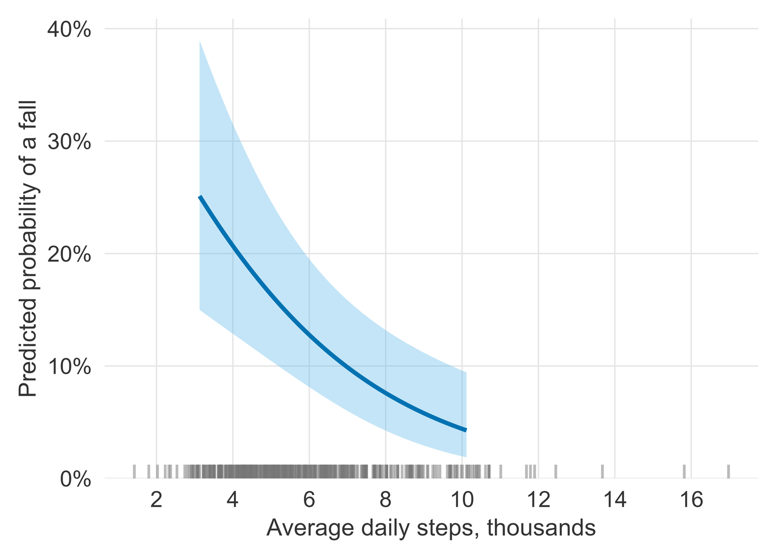
How to read it: the line is the predicted probability of a fall for one reference participant, described in the caption, as only her daily steps change; the band is the 95% CI of that prediction. For this reference participant the model gives 25.1% (95% CI 15.0% to 38.9%) at 3.1 thousand steps a day and 4.3% (1.9% to 9.4%) at 10.1 thousand. The curve is drawn only between the 5th and 95th percentiles of observed steps, so it does not run into the sparse tails; the ticks along the bottom show every participant, tails included. Other reference values give a curve at a different height and steepness, while the adjusted odds ratio stays the same, which is why the reference values are always stated.วิธีอ่าน: เส้นคือความน่าจะเป็นของการหกล้มที่ทำนายสำหรับผู้เข้าร่วมอ้างอิงหนึ่งคนตามที่ระบุในคำบรรยายรูป เมื่อเปลี่ยนเฉพาะจำนวนก้าวต่อวัน แถบคือช่วงความเชื่อมั่น 95% ของค่าทำนายนั้น สำหรับผู้เข้าร่วมอ้างอิงคนนี้ แบบจำลองให้ค่า 25.1% (95% CI 15.0% ถึง 38.9%) ที่ 3.1 พันก้าวต่อวัน และ 4.3% (1.9% ถึง 9.4%) ที่ 10.1 พันก้าวต่อวัน วาดเส้นเฉพาะช่วงเปอร์เซ็นไทล์ที่ 5 ถึง 95 ของจำนวนก้าวที่สังเกตได้ จึงไม่ลากเข้าไปในช่วงปลายที่มีข้อมูลน้อย ส่วนขีดตามแนวล่างแสดงผู้เข้าร่วมทุกคน รวมทั้งช่วงปลาย ค่าอ้างอิงชุดอื่นจะให้เส้นที่สูงต่ำและความชันต่างออกไป ขณะที่ adjusted odds ratio ยังคงเท่าเดิม จึงต้องระบุค่าอ้างอิงทุกครั้ง
Does a new marker add information? The add-on model comparisonตัวบ่งชี้ใหม่ให้ข้อมูลเพิ่มหรือไม่: การเปรียบเทียบแบบจำลองเมื่อเพิ่มตัวบ่งชี้
Why the likelihood-ratio test is the primary evidence. Asking whether the marker adds information is asking whether its coefficient is zero once the base variables are in the model, and the likelihood-ratio test answers exactly that. The change in AUC is an insensitive measure: when the base model already ranks people who fall above people who do not reasonably well, even a marker with a clear independent association moves the AUC only a little. The DeLong test is also not designed for two nested models fitted to the same data, where it is known to be conservative and gives P values that are too large; the same caveat applies to its confidence interval for the change in AUC.เหตุผลที่ใช้ likelihood-ratio test เป็นหลักฐานหลัก คำถามว่าตัวบ่งชี้ให้ข้อมูลเพิ่มจากแบบจำลองพื้นฐานหรือไม่ ก็คือคำถามว่าสัมประสิทธิ์ของตัวบ่งชี้เท่ากับศูนย์หรือไม่เมื่อมีตัวแปรพื้นฐานอยู่ในแบบจำลองแล้ว ซึ่ง likelihood-ratio test ตอบได้โดยตรง ส่วนการเปลี่ยนแปลงของ AUC เป็นตัววัดที่ไม่ไว (insensitive) เมื่อแบบจำลองพื้นฐานจัดลำดับผู้ที่หกล้มให้สูงกว่าผู้ที่ไม่หกล้มได้ค่อนข้างดีอยู่แล้ว แม้ตัวบ่งชี้ที่มีความสัมพันธ์อิสระชัดเจนก็ทำให้ AUC เปลี่ยนไปเพียงเล็กน้อย นอกจากนี้ DeLong test ไม่ได้ออกแบบมาสำหรับแบบจำลองซ้อนกัน (nested models) สองแบบที่สร้างจากข้อมูลชุดเดียวกัน ในสถานการณ์นี้ทราบกันว่าการทดสอบให้ผลแบบ conservative คือให้ค่า P สูงเกินจริง ข้อจำกัดเดียวกันนี้ใช้กับช่วงความเชื่อมั่นของการเปลี่ยนแปลง AUC ด้วย
| Measure | Base model | Base + timed up-and-go | Comparison |
|---|---|---|---|
| Coefficients, excluding the intercept | 7 | 8 | +1 |
| Timed up-and-go, OR per second (95% CI) | Not in the model | 1.37 (1.17 to 1.61) | |
| Log-likelihood | −203.70 | −196.07 | LR chi-square 15.27, 1 df, P <0.001 |
| AIC (lower is better) | 423.4 | 410.1 | Change −13.3 |
| Apparent AUC (95% CI) | 0.735 (0.676 to 0.794) | 0.759 (0.704 to 0.814) | Change 0.024 (−0.004 to 0.052), DeLong P = 0.092 |
- Base model: the adjusted logistic model of Table 1. OR, odds ratio per second of timed up-and-go time, with its profile-likelihood 95% CI.แบบจำลองพื้นฐานคือแบบจำลองโลจิสติกที่ปรับแล้วในตารางที่ 1 OR คือ odds ratio ต่อเวลาในการทดสอบ Timed Up and Go ที่เพิ่มขึ้นหนึ่งวินาที พร้อม 95% CI แบบ profile likelihood
- LR, likelihood ratio; df, degrees of freedom; AIC, Akaike information criterion; AUC, area under the ROC curve.LR คือ likelihood ratio, df คือองศาอิสระ, AIC คือ Akaike information criterion และ AUC คือพื้นที่ใต้เส้นโค้ง ROC
- The AUC values are apparent (measured on the data used to fit the models), with DeLong 95% CI; the change and its DeLong test compare the two models in the same participants.ค่า AUC เป็นแบบ apparent (วัดจากข้อมูลชุดเดียวกับที่ใช้สร้างแบบจำลอง) พร้อม 95% CI ด้วยวิธี DeLong การเปลี่ยนแปลงของ AUC และ DeLong test เปรียบเทียบสองแบบจำลองในผู้เข้าร่วมกลุ่มเดียวกัน
How to read it: adding the timed up-and-go test gave an odds ratio of 1.37 per second (95% CI 1.17 to 1.61) and a likelihood-ratio chi-square of 15.27 on 1 df, P value <0.001; AIC changed by −13.3. The apparent AUC went from 0.735 to 0.759, a change of 0.024 (95% CI −0.004 to 0.052, DeLong P value 0.092). This is the pattern described above: a small likelihood-ratio P value next to an AUC change whose interval includes zero. The extended model has 12.8 events per coefficient.วิธีอ่าน: การเพิ่มผลการทดสอบ Timed Up and Go ให้ odds ratio เท่ากับ 1.37 ต่อวินาที (95% CI 1.17 ถึง 1.61) likelihood-ratio chi-square เท่ากับ 15.27 ที่องศาอิสระ 1 (ค่า P <0.001) และค่า AIC เปลี่ยนไป −13.3 ส่วน AUC แบบ apparent เปลี่ยนจาก 0.735 เป็น 0.759 หรือเปลี่ยนไป 0.024 (95% CI −0.004 ถึง 0.052 ค่า P จาก DeLong test 0.092) ซึ่งเป็นรูปแบบตามที่อธิบายไว้ข้างต้น คือ likelihood-ratio test ให้ค่า P น้อย ขณะที่ช่วงความเชื่อมั่นของการเปลี่ยนแปลง AUC ครอบคลุมศูนย์ แบบจำลองขยายมีจำนวนเหตุการณ์ต่อสัมประสิทธิ์เท่ากับ 12.8
Assumption checksการตรวจสอบข้อตกลงเบื้องต้นของแบบจำลอง
| Check | Logistic model: fall | Linear model: walk distance |
|---|---|---|
| Model size | ||
| Events or participants per coefficient | 14.6 (102 events / 7) | 52.5 (420 participants / 8) |
| Collinearity: variance inflation factor | ||
| Daily steps | 1.16 | 1.44 |
| Age | 1.01 | 1.17 |
| Sex | 1.04 | 1.12 |
| Body-mass index | 1.06 | 1.10 |
| Self-rated health* | 1.08 | 1.19 |
| Knee or hip pain | 1.10 | 1.23 |
| Walk distance at enrolment | Not in the model | 1.90 |
| Linearity: restricted cubic spline against a straight line, P | ||
| Daily steps | 0.319 | 0.014 |
| Age | 0.077 | 0.487 |
| Body-mass index | 0.451 | 0.795 |
| Walk distance at enrolment | Not in the model | 0.472 |
| Residuals of the linear model | ||
| Breusch-Pagan score test of constant variance, P | Not applicable | 0.222 |
| Studentized residuals beyond ±3, n (expected if normal) | Not applicable | 0 (1.1) |
| Skewness of the residuals | Not applicable | −0.04 |
- Model size: participants with a fall divided by the coefficients the logistic model estimates, intercept excluded; for the linear model, all participants divided by its coefficients.ขนาดของแบบจำลอง: จำนวนผู้ที่หกล้มหารด้วยจำนวนสัมประสิทธิ์ที่แบบจำลองโลจิสติกประมาณ (ไม่นับค่าคงที่) สำหรับแบบจำลองเชิงเส้นใช้จำนวนผู้เข้าร่วมทั้งหมดหารด้วยจำนวนสัมประสิทธิ์
- Collinearity: generalised variance inflation factors (GVIF), equal to the usual VIF for a variable with one coefficient. * Self-rated health enters as 2 indicator terms and its GVIF covers them together; for such a variable GVIF^(1/(2·df)) is the value comparable with the square root of a one-coefficient VIF (here 1.02 in the logistic model and 1.04 in the linear model).ภาวะร่วมเส้นตรงพหุ (collinearity): ค่า generalised variance inflation factor (GVIF) ซึ่งเท่ากับ VIF ปกติสำหรับตัวแปรที่มีสัมประสิทธิ์ตัวเดียว * ภาวะสุขภาพที่ประเมินด้วยตนเองเข้าสู่แบบจำลองเป็นตัวแปรหุ่น (indicator) 2 ตัว และค่า GVIF ครอบคลุมตัวแปรหุ่นทุกตัวพร้อมกัน สำหรับตัวแปรลักษณะนี้ ค่า GVIF^(1/(2·df)) คือค่าที่เทียบได้กับรากที่สองของ VIF ของตัวแปรที่มีสัมประสิทธิ์ตัวเดียว (ในตัวอย่างนี้เท่ากับ 1.02 ในแบบจำลองโลจิสติก และ 1.04 ในแบบจำลองเชิงเส้น)
- Linearity: each continuous covariate refitted as a restricted (natural) cubic spline with 4 knots (3 degrees of freedom in total) and compared with the straight-line model on 2 degrees of freedom by a likelihood-ratio test (logistic) or an F test (linear).ความเป็นเส้นตรง: ใส่ตัวแปรต่อเนื่องแต่ละตัวใหม่ในรูป restricted (natural) cubic spline ที่มี 4 knot (รวม 3 องศาอิสระ) แล้วเปรียบเทียบกับแบบจำลองเส้นตรงที่องศาอิสระ 2 ด้วย likelihood-ratio test (โลจิสติก) หรือ F test (เชิงเส้น)
- Residuals: Breusch-Pagan (Cook-Weisberg) score test of constant variance against the fitted values; studentized residuals beyond ±3, with the number expected if the errors were normal in brackets; skewness of the residuals, zero for a symmetric spread.ค่าส่วนเหลือ: Breusch-Pagan (Cook-Weisberg) score test ของความแปรปรวนคงที่เทียบกับค่าที่ทำนาย จำนวน studentized residual ที่เกิน ±3 โดยในวงเล็บคือจำนวนที่คาดไว้หากค่าคลาดเคลื่อนแจกแจงแบบปกติ และความเบ้ของค่าส่วนเหลือ ซึ่งเป็นศูนย์เมื่อการกระจายสมมาตร
How to read it: a common rough guide asks for at least 10 events per coefficient in a logistic model (here 14.6); it is only rough, and a formal sample-size calculation for the model is better. A variance inflation factor near one means a variable shares little information with the others, and values above about 5 deserve a closer look; the largest here are 1.16 in the logistic model and 1.90 in the linear model. In the linearity rows, a small P value is evidence that a straight line may miss a curve.วิธีอ่าน: แนวทางคร่าว ๆ ที่ใช้กันทั่วไปต้องการจำนวนเหตุการณ์อย่างน้อย 10 ต่อสัมประสิทธิ์ในแบบจำลองโลจิสติก (ในตัวอย่างนี้เท่ากับ 14.6) แนวทางนี้เป็นเพียงเกณฑ์คร่าว ๆ การคำนวณขนาดตัวอย่างสำหรับแบบจำลองอย่างเป็นทางการจะดีกว่า ค่า variance inflation factor ที่ใกล้หนึ่งหมายถึงตัวแปรนั้นมีข้อมูลซ้ำซ้อนกับตัวแปรอื่นน้อย ค่าที่สูงกว่าประมาณ 5 ควรพิจารณาให้ละเอียดขึ้น ค่าสูงสุดในตัวอย่างนี้คือ 1.16 ในแบบจำลองโลจิสติก และ 1.90 ในแบบจำลองเชิงเส้น ในแถวความเป็นเส้นตรง ค่า P ที่น้อยเป็นหลักฐานว่าเส้นตรงอาจไม่สามารถจับความโค้งของความสัมพันธ์ได้
One check is flagged: daily steps in the linear model, where the spline comparison gives P value 0.014 (in the logistic model the same comparison gives 0.319). In a delivered job a flag like this is reported, not hidden: the report shows the spline curve beside the straight line, gives the results of the model with the spline as a sensitivity analysis, and the research team decides which model to report. With this many checks one small P value can also arise by chance, which is why the curve is looked at and not only the P value.มีการตรวจหนึ่งรายการที่พบสัญญาณผิดปกติ คือจำนวนก้าวต่อวันในแบบจำลองเชิงเส้น ซึ่งการเปรียบเทียบกับ spline ให้ค่า P 0.014 (ในแบบจำลองโลจิสติก การเปรียบเทียบเดียวกันให้ค่า 0.319) ในงานจริงที่ส่งมอบ สัญญาณลักษณะนี้ต้องรายงาน ไม่ซ่อนไว้ โดยรายงานจะแสดงเส้นโค้ง spline เทียบกับเส้นตรง ให้ผลของแบบจำลองที่ใช้ spline เป็นการวิเคราะห์ความไว (sensitivity analysis) และให้ทีมวิจัยตัดสินใจว่าจะรายงานแบบจำลองใด เมื่อมีการตรวจหลายรายการเช่นนี้ ค่า P ที่น้อยหนึ่งค่าอาจเกิดจากความบังเอิญได้ จึงต้องดูรูปร่างของเส้นโค้งประกอบ ไม่ดูเพียงค่า P
What this sample does not show: the AUC values are apparent, with no internal validation or optimism correction; there are no missing data, no interaction terms and no sensitivity analysis for unmeasured confounding; and the add-on comparison measures statistical information, not whether using the test would change care. What these results mean for older adults, and what to do about them, is for the research team to interpret.สิ่งที่ตัวอย่างนี้ไม่ได้แสดง: ค่า AUC เป็นแบบ apparent โดยไม่มีการตรวจสอบความถูกต้องภายใน (internal validation) หรือการปรับแก้ optimism ไม่มีข้อมูลที่ขาดหาย ไม่มีพจน์ปฏิสัมพันธ์ (interaction) และไม่มีการวิเคราะห์ความไวต่อตัวแปรกวนที่ไม่ได้วัด นอกจากนี้การเปรียบเทียบเมื่อเพิ่มตัวบ่งชี้วัดเพียงข้อมูลทางสถิติที่เพิ่มขึ้น ไม่ได้บอกว่าการใช้การทดสอบนี้จะเปลี่ยนแนวทางการดูแลผู้สูงอายุหรือไม่ ความหมายของผลเหล่านี้ต่อผู้สูงอายุ และสิ่งที่ควรทำต่อ เป็นหน้าที่ของทีมวิจัยในการแปลผล
What you send and do yourselfสิ่งที่คุณต้องส่งและทำเอง
- Your research question, with the exposure, the outcome and the variables you consider confounders.คำถามวิจัย พร้อมระบุปัจจัยที่ศึกษา ผลลัพธ์ และตัวแปรที่คุณเห็นว่าเป็นตัวแปรกวน
- A de-identified dataset with its codebook: no names, ID numbers, addresses or anything else that identifies a person.ชุดข้อมูลที่ตัดข้อมูลระบุตัวตนออกแล้ว พร้อมคู่มือรหัสตัวแปร (codebook) โดยไม่มีชื่อ เลขประจำตัว ที่อยู่ หรือข้อมูลอื่นที่ระบุตัวบุคคลได้
- You interpret the results and write your own article, and acknowledge the statistical help in the way your journal asks.คุณเป็นผู้แปลผลและเขียนบทความของคุณเอง และระบุความช่วยเหลือด้านสถิติตามรูปแบบที่วารสารกำหนด
Limitsขอบเขตและข้อจำกัด
- Statistical analysis and advice only: the research question, the data, the interpretation and the writing stay yours.บริการนี้เป็นงานวิเคราะห์และให้คำแนะนำทางสถิติเท่านั้น คำถามวิจัย ข้อมูล การแปลผล และการเขียน เป็นของคุณทั้งหมด
- Choosing confounders needs your subject knowledge: I advise on the choice, but never pick variables to reach a wanted result.การเลือกตัวแปรกวนต้องอาศัยความรู้ในสาขาของคุณ ผมให้คำแนะนำได้ แต่จะไม่เลือกตัวแปรเพื่อให้ได้ผลตามที่ต้องการ
- Not for a thesis, an independent study or other work submitted for a degree; for those, I offer consultation only.ไม่รับทำงานที่จะนำไปใช้เพื่อสำเร็จการศึกษา เช่น วิทยานิพนธ์ การค้นคว้าอิสระ หรือผลงานอื่นที่ยื่นเพื่อรับปริญญา งานลักษณะนี้รับเฉพาะการให้คำปรึกษา
- Authorship is not sold and is not a condition of the service.การมีชื่อเป็นผู้นิพนธ์ไม่ใช่สิ่งที่ซื้อขายได้ และไม่ใช่เงื่อนไขในการรับงาน
Request this serviceขอใช้บริการนี้
Every request is reviewed first. I may accept or decline it. The timeline is agreed per project after review.ผมพิจารณาคำขอทุกงานก่อน และอาจรับหรือปฏิเสธงาน ระยะเวลาของแต่ละงานตกลงกันหลังพิจารณาคำขอแล้ว
Member prices apply only to orders that start on uniqcret.com; if you found me on Fastwork or your enquiry began there, please order on Fastwork at the Fastwork price.ราคาสมาชิกใช้กับงานที่เริ่มต้นบน uniqcret.com เท่านั้น หากคุณรู้จักผมจาก Fastwork หรือเริ่มสอบถามบน Fastwork กรุณาสั่งงานบน Fastwork ในราคาของ Fastwork