Mixed models for repeated measuresแบบจำลองผสมสำหรับข้อมูลวัดซ้ำ
Mixed models for repeated measures in a two-arm studyแบบจำลองผลกระทบผสม (mixed model) สำหรับข้อมูลที่วัดซ้ำในการศึกษาสองกลุ่ม
An invented community health centre ran a randomised two-arm study of a guided group exercise programme against usual care (a leaflet of home exercises) in 120 inactive adults: 60 in the exercise arm and 60 in usual care. The outcome is the six-minute walk distance in metres, measured at baseline and at 3 follow-up visits, at weeks 4, 8 and 12. Walks of the same person are correlated, because some people walk further than others at every visit. By week 12, 22 people (18%) had left the study; in the simulation, a shorter walk at one visit made leaving before the next visit more likely. The data were simulated with no difference between the arms at baseline and a true difference that grows to 15, 30 and 45 m at the follow-up visits. The centre, the people and every value are invented: all data are simulated with a fixed seed.ศูนย์สุขภาพชุมชนสมมุติแห่งหนึ่งทำการศึกษาแบบสุ่มสองกลุ่ม เปรียบเทียบโปรแกรมออกกำลังกายแบบกลุ่มที่มีผู้ฝึกดูแล กับการดูแลตามปกติ (แผ่นพับท่าออกกำลังกายที่บ้าน) ในผู้ใหญ่ที่มีกิจกรรมทางกายน้อย 120 คน แบ่งเป็นกลุ่มออกกำลังกาย 60 คน และกลุ่มดูแลตามปกติ 60 คน ผลลัพธ์คือระยะทางที่เดินได้ในหกนาที (six-minute walk distance) หน่วยเป็นเมตร วัดที่ baseline และวัดติดตามอีก 3 ครั้ง ที่สัปดาห์ 4, 8 และ 12 ค่าที่วัดซ้ำในคนเดียวกันมีความสัมพันธ์กัน เพราะบางคนเดินได้ไกลกว่าคนอื่นในทุกครั้งที่วัด เมื่อถึงสัปดาห์ที่ 12 มีผู้ออกจากการศึกษาไปแล้ว 22 คน (18%) และในการจำลอง ผู้ที่เดินได้ระยะสั้นในครั้งหนึ่งมีโอกาสออกจากการศึกษาก่อนการวัดครั้งถัดไปมากกว่า ข้อมูลถูกจำลองโดยกำหนดให้ไม่มีความแตกต่างระหว่างกลุ่มที่ baseline และให้ความแตกต่างจริงเพิ่มขึ้นเป็น 15, 30 และ 45 เมตรในการวัดติดตามแต่ละครั้ง ศูนย์สุขภาพ ผู้เข้าร่วม และค่าทุกค่าเป็นเรื่องสมมุติ ข้อมูลทั้งหมดเป็นข้อมูลจำลองที่สร้างด้วย seed คงที่
What you receiveสิ่งที่คุณจะได้รับ
Analysis of an outcome measured several times on the same people, using a mixed model that keeps every available visit. This is valid when missing visits are missing at random; that assumption is stated, and a sensitivity analysis shows how much the results depend on it.วิเคราะห์ผลลัพธ์ที่วัดซ้ำหลายครั้งในคนเดิม ด้วยแบบจำลองผสม (mixed model) ที่ใช้ข้อมูลจากทุกครั้งที่มีการวัด วิธีนี้ให้ผลถูกต้องเมื่อข้อมูลที่ขาดหายเป็นแบบ missing at random ซึ่งจะระบุสมมติฐานนี้ไว้ และใช้การวิเคราะห์ความไว (sensitivity analysis) แสดงว่าผลขึ้นกับสมมติฐานนี้มากน้อยเพียงใด
- A profile plot of each group over time.กราฟแสดงแนวโน้มของแต่ละกลุ่มตามเวลา
- The mixed-model table, with the covariance structure stated.ตารางแบบจำลองผสม พร้อมระบุโครงสร้างความแปรปรวนร่วมที่ใช้
- Estimates at each visit and between-group contrasts, each with a 95% confidence interval.ค่าประมาณในแต่ละครั้งที่วัด และผลต่างระหว่างกลุ่ม พร้อมช่วงความเชื่อมั่น 95%
- A record of the model checks.บันทึกผลการตรวจสอบแบบจำลอง
The sampleตัวอย่างงาน
Sample work on simulated data. No real patient, no client project.ตัวอย่างงานจากข้อมูลจำลองทั้งหมด ไม่ใช่ข้อมูลผู้ป่วยจริง และไม่ใช่งานของลูกค้ารายใด
What this sample containsสิ่งที่อยู่ในตัวอย่างนี้
- A profile plot of the observed mean and 95% confidence interval by arm and visit, with the number of people measured at each visit under the axis.กราฟโปรไฟล์ (profile plot) แสดงค่าเฉลี่ยที่สังเกตได้และช่วงความเชื่อมั่น 95% แยกตามกลุ่มและครั้งที่วัด พร้อมจำนวนผู้ที่ได้รับการวัดในแต่ละครั้งใต้แกนนอน
- The model written out in words, with the reason it was chosen.คำอธิบายแบบจำลองครบทุกส่วน พร้อมเหตุผลที่เลือกใช้
- A model table: fixed effects with 95% confidence intervals, the between-person and residual standard deviations, and the ICC.ตารางแบบจำลอง: fixed effects พร้อมช่วงความเชื่อมั่น 95% ส่วนเบี่ยงเบนมาตรฐานระหว่างบุคคลและของความคลาดเคลื่อน (residual) และค่า ICC
- Estimated means by arm at each follow-up visit and the difference between the arms with 95% confidence intervals, set beside the true differences of the simulation, with the primary contrast marked and the degrees-of-freedom method named.ค่าเฉลี่ยที่ประมาณจากแบบจำลองของแต่ละกลุ่มในการวัดติดตามแต่ละครั้ง และความแตกต่างระหว่างกลุ่มพร้อมช่วงความเชื่อมั่น 95% วางเทียบกับความแตกต่างจริงของการจำลอง โดยระบุ contrast หลักและวิธีคำนวณองศาอิสระ (degrees of freedom)
- What missing at random means for this study, and a small table setting the model estimate beside two complete-case analyses at the last visit: a t-test and a baseline-adjusted analysis.ความหมายของข้อมูลขาดหายแบบสุ่ม (missing at random) สำหรับการศึกษานี้ และตารางเล็กที่วางค่าประมาณจากแบบจำลองเทียบกับการวิเคราะห์เฉพาะผู้ที่มีข้อมูลในครั้งสุดท้าย (complete case) สองวิธี คือ t-test และการวิเคราะห์ที่ปรับด้วยค่า baseline
- A methods paragraph to adapt for a manuscript, a note on how to read each table and figure, and the limits.ย่อหน้าวิธีการทางสถิติสำหรับปรับใช้ในต้นฉบับบทความ คำอธิบายวิธีอ่านตารางและรูปแต่ละชิ้น และข้อจำกัด
The observed dataข้อมูลที่สังเกตได้
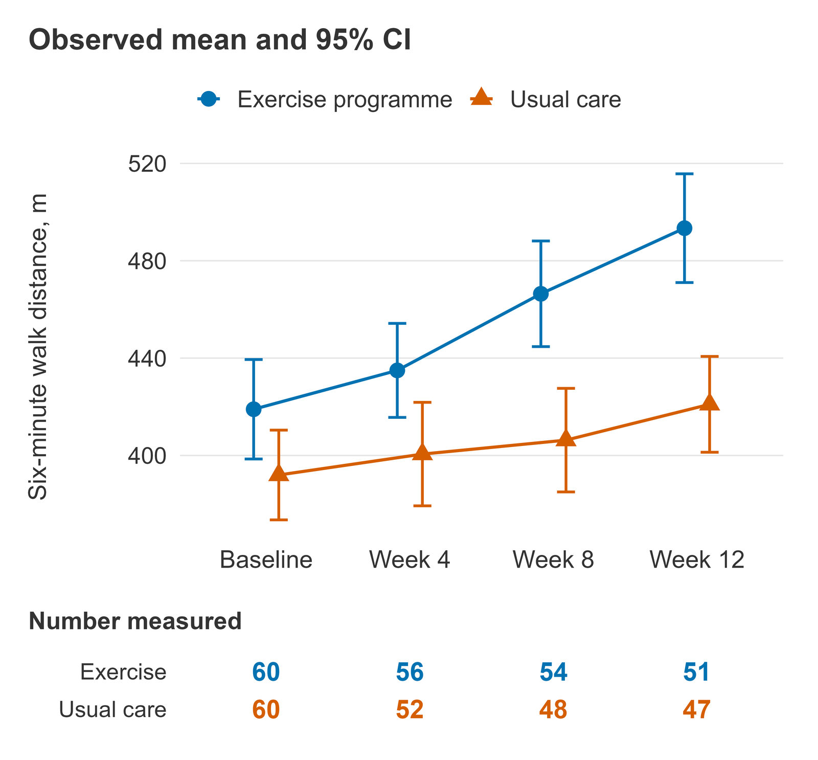
How to read it: each point is the mean of the people measured at that visit, and the bar is its 95% confidence interval. The plot shows the data as observed: from week 4 on, each mean uses only the people still in the study, so it can drift upward when people with shorter walks leave. The arms also differ at baseline by chance (419 m in the exercise arm against 392 m in usual care); the model below compares people with the same baseline walk, so it adjusts for this chance difference. The numbers under the axis show how many people each mean rests on: at week 12, 51 in the exercise arm and 47 in usual care.วิธีอ่าน: แต่ละจุดคือค่าเฉลี่ยของผู้ที่ได้รับการวัดในครั้งนั้น และแถบแนวตั้งคือช่วงความเชื่อมั่น 95% ของค่าเฉลี่ยนั้น กราฟนี้แสดงข้อมูลตามที่สังเกตได้จริง ตั้งแต่สัปดาห์ที่ 4 เป็นต้นไป ค่าเฉลี่ยแต่ละค่าคำนวณจากผู้ที่ยังอยู่ในการศึกษาเท่านั้น จึงอาจสูงขึ้นได้เมื่อผู้ที่เดินได้ระยะสั้นออกจากการศึกษาไป นอกจากนี้ สองกลุ่มยังต่างกันตั้งแต่ baseline โดยบังเอิญ (419 เมตรในกลุ่มออกกำลังกาย เทียบกับ 392 เมตรในกลุ่มดูแลตามปกติ) แบบจำลองด้านล่างเปรียบเทียบคนที่มีระยะทางเดินที่ baseline เท่ากัน แบบจำลองจึงปรับความแตกต่างโดยบังเอิญนี้ไว้แล้ว ตัวเลขใต้แกนบอกว่าค่าเฉลี่ยแต่ละค่ามาจากผู้เข้าร่วมกี่คน ที่สัปดาห์ที่ 12 เหลือ 51 คนในกลุ่มออกกำลังกาย และ 47 คนในกลุ่มดูแลตามปกติ
The modelแบบจำลอง
The walk distance of each person at each follow-up visit (weeks 4, 8 and 12) is modelled as: intercept + arm + visit + arm-by-visit interaction + baseline walk distance + a random intercept for the person + a residual. Visit is categorical, so the model sets no shape for the change over time, and the arm-by-visit interaction lets the difference between the arms take its own value at each visit. The baseline walk enters as a covariate, centred at the mean of all 120 randomised people (405.5 m). The random intercept, assumed normal with mean zero, lets each person sit above or below the average at every visit, which is what makes the visits of one person correlated; the residual, also assumed normal, is the visit-to-visit variation within a person. The model was fitted by restricted maximum likelihood (REML).แบบจำลองกำหนดให้ระยะทางเดินของแต่ละคนในการวัดติดตามแต่ละครั้ง (สัปดาห์ที่ 4, 8 และ 12) เท่ากับ ค่าคงที่ (intercept) + กลุ่ม + ครั้งที่วัด + ปฏิสัมพันธ์ระหว่างกลุ่มกับครั้งที่วัด (arm-by-visit interaction) + ระยะทางเดินที่ baseline + ค่าคงที่สุ่ม (random intercept) ของแต่ละคน + ความคลาดเคลื่อน (residual) ครั้งที่วัดใส่เป็นตัวแปรเชิงกลุ่ม (categorical) แบบจำลองจึงไม่ได้กำหนดรูปแบบของการเปลี่ยนแปลงตามเวลาไว้ล่วงหน้า และพจน์ปฏิสัมพันธ์ทำให้ความแตกต่างระหว่างกลุ่มมีค่าเฉพาะของตนเองในแต่ละครั้ง ระยะทางเดินที่ baseline ใส่เป็นตัวแปรร่วม (covariate) โดยลบด้วยค่าเฉลี่ย (centring) ของผู้ถูกสุ่มทั้ง 120 คน (405.5 เมตร) ค่าคงที่สุ่มซึ่งสมมุติให้แจกแจงแบบปกติและมีค่าเฉลี่ยเป็นศูนย์ ทำให้แต่ละคนอยู่สูงหรือต่ำกว่าค่าเฉลี่ยในทุกครั้งที่วัด ซึ่งเป็นที่มาของสหสัมพันธ์ระหว่างค่าที่วัดซ้ำในคนเดียวกัน ส่วนความคลาดเคลื่อนซึ่งสมมุติให้แจกแจงแบบปกติเช่นกัน คือความผันแปรระหว่างครั้งภายในคนเดียวกัน ประมาณค่าแบบจำลองด้วยวิธี restricted maximum likelihood (REML)
Why this model: a random-intercept mixed model was chosen because it uses every visit a person attended and separates the between-person from the within-person variation, which gives the ICC. Kenward-Roger standard errors and degrees of freedom were used so that the intervals allow for the variance components being estimated. Because the model assumes that any two visits of the same person are equally correlated, the primary contrast was re-estimated with an unstructured covariance (the usual repeated-measures model of a trial, often called MMRM), which makes no such assumption.เหตุผลที่เลือกแบบจำลองนี้: เลือก mixed model ที่มีค่าคงที่สุ่ม (random intercept) เพราะใช้ข้อมูลทุกครั้งที่แต่ละคนมาวัด และแยกความแปรปรวนระหว่างบุคคลออกจากความแปรปรวนภายในบุคคล จึงได้ค่า ICC ใช้ค่าความคลาดเคลื่อนมาตรฐานและองศาอิสระแบบ Kenward-Roger เพื่อให้ช่วงความเชื่อมั่นคำนึงถึงความไม่แน่นอนจากการประมาณองค์ประกอบความแปรปรวน และเนื่องจากแบบจำลองนี้สมมุติว่าค่าสองครั้งใด ๆ ของคนเดียวกันมีสหสัมพันธ์เท่ากันเสมอ จึงประมาณ contrast หลักซ้ำด้วยแบบจำลองที่ใช้เมทริกซ์ความแปรปรวนร่วมแบบไม่มีโครงสร้าง (unstructured covariance) ซึ่งเป็นแบบจำลองการวัดซ้ำที่นิยมใช้ในการทดลองทางคลินิก (มักเรียกว่า MMRM) และไม่ได้สมมุติเช่นนั้น
| Term | Estimate | 95% CI* |
|---|---|---|
| Fixed effects, m | ||
| Intercept: usual care, week 4 | 406.1 | 394.3 to 418.0 |
| Exercise vs usual care, week 4 | 15.1 | −1.5 to 31.7 |
| Week 8 vs week 4, usual care | −1.3 | −12.6 to 10.1 |
| Week 12 vs week 4, usual care | 12.8 | 1.4 to 24.3 |
| Baseline walk, per metre | 0.84 | 0.74 to 0.93 |
| Arm by visit: week 8 | 31.9 | 16.3 to 47.6 |
| Arm by visit: week 12 | 39.4 | 23.5 to 55.2 |
| Random part | ||
| Between-person SD (random intercept), m | 32.6 | 27.0 to 38.2 |
| Residual SD (within person), m | 28.5 | 25.6 to 31.2 |
| ICC | 0.57 | |
- * Fixed effects: 95% confidence interval from the t distribution with Kenward-Roger standard errors and degrees of freedom. Standard deviations: profile 95% confidence interval. No interval is given for the ICC.* fixed effects: ช่วงความเชื่อมั่น 95% คำนวณจากการแจกแจง t โดยใช้ค่าความคลาดเคลื่อนมาตรฐานและองศาอิสระแบบ Kenward-Roger ส่วนเบี่ยงเบนมาตรฐานใช้ช่วงความเชื่อมั่นแบบ profile และไม่ได้คำนวณช่วงความเชื่อมั่นของ ICC
- The intercept is the mean in usual care at week 4 for a person with the average baseline walk. The row Exercise vs usual care, week 4 is the difference between the arms at that visit; each arm-by-visit row is how much larger the difference between the arms is at that visit than at week 4.ค่าคงที่ (intercept) คือค่าเฉลี่ยของกลุ่มดูแลตามปกติที่สัปดาห์ที่ 4 สำหรับคนที่มีระยะทางเดินที่ baseline เท่าค่าเฉลี่ย แถว Exercise vs usual care, week 4 คือความแตกต่างระหว่างกลุ่มในครั้งนั้น และแถว arm by visit แต่ละแถวคือส่วนต่างของความแตกต่างระหว่างกลุ่มในครั้งนั้น เทียบกับที่สัปดาห์ที่ 4
- The model uses 308 follow-up visits from 108 people; 12 people left before the first follow-up visit and have no follow-up value to model.แบบจำลองใช้ข้อมูลการวัดติดตาม 308 ครั้งจากผู้เข้าร่วม 108 คน มีผู้เข้าร่วม 12 คนที่ออกจากการศึกษาก่อนการวัดติดตามครั้งแรก จึงไม่มีค่าในการวัดติดตามให้นำเข้าแบบจำลอง
- SD, standard deviation. ICC, intraclass correlation coefficient: the share of the variation left after adjusting for the baseline walk that lies between people.SD คือส่วนเบี่ยงเบนมาตรฐาน ICC คือสัมประสิทธิ์สหสัมพันธ์ภายในชั้น (intraclass correlation coefficient) หมายถึงสัดส่วนของความแปรปรวนระหว่างบุคคล ในความแปรปรวนทั้งหมดที่เหลือหลังปรับด้วยระยะทางเดินที่ baseline
How to read it: the baseline coefficient, 0.84, means that a person who walked one metre further at baseline walked on average 0.84 m further at follow-up, in either arm. After that adjustment people still differ: the between-person SD is 32.6 m, and the residual SD, the variation of one person from visit to visit, is 28.5 m. The ICC of 0.57 is the model's estimate of the correlation between any two follow-up visits of the same person after adjusting for the baseline walk; the model assumes this correlation is the same for every pair of visits (the unstructured check below estimated 0.52 to 0.61). The difference between the arms at each visit is easier to read in the next table than from the interaction rows.วิธีอ่าน: สัมประสิทธิ์ของ baseline เท่ากับ 0.84 หมายความว่าผู้ที่เดินได้ไกลกว่าหนึ่งเมตรที่ baseline จะเดินได้ไกลกว่าโดยเฉลี่ย 0.84 เมตรในการวัดติดตาม ไม่ว่าจะอยู่กลุ่มใด หลังปรับด้วย baseline แล้วแต่ละคนยังคงแตกต่างกัน โดยส่วนเบี่ยงเบนมาตรฐานระหว่างบุคคลเท่ากับ 32.6 เมตร และส่วนเบี่ยงเบนมาตรฐานของความคลาดเคลื่อน ซึ่งคือความผันแปรของคนคนเดียวกันระหว่างครั้งที่วัด เท่ากับ 28.5 เมตร ค่า ICC เท่ากับ 0.57 คือค่าประมาณสหสัมพันธ์ระหว่างการวัดติดตามสองครั้งใด ๆ ของคนเดียวกันหลังปรับด้วยระยะทางเดินที่ baseline โดยแบบจำลองสมมุติว่าสหสัมพันธ์นี้เท่ากันทุกคู่ของครั้งที่วัด (แบบจำลองแบบไม่มีโครงสร้างด้านล่างประมาณได้ 0.52 ถึง 0.61) ความแตกต่างระหว่างกลุ่มในแต่ละครั้งอ่านจากตารางถัดไปได้ง่ายกว่าอ่านจากแถวปฏิสัมพันธ์
Estimated means and differences at each visitค่าเฉลี่ยที่ประมาณได้และความแตกต่างในแต่ละครั้งที่วัด
| Visit | Estimated mean (95% CI), m | Exercise minus usual care (95% CI), m | True difference, m | |
|---|---|---|---|---|
| Exercise programme | Usual care | |||
| Week 4 | 421.2 (409.7 to 432.7) | 406.1 (394.3 to 418.0) | 15.1 (−1.5 to 31.7) | 15 |
| Week 8 | 451.9 (440.2 to 463.5) | 404.9 (392.7 to 417.0) | 47.0 (30.1 to 63.9) | 30 |
| Week 12* | 473.4 (461.5 to 485.3) | 419.0 (406.7 to 431.2) | 54.5 (37.4 to 71.5) | 45 |
- * Primary contrast: the difference between the arms at week 12, the end of the programme.* contrast หลัก: ความแตกต่างระหว่างกลุ่มที่สัปดาห์ที่ 12 ซึ่งเป็นช่วงสิ้นสุดโปรแกรม
- Estimated marginal means are for a person with the average baseline walk of all randomised people (405.5 m). The difference is exercise minus usual care: a positive value means a longer walk in the exercise arm.ค่าเฉลี่ยที่ประมาณได้ (estimated marginal means) คำนวณสำหรับคนที่มีระยะทางเดินที่ baseline เท่าค่าเฉลี่ยของผู้ถูกสุ่มทุกคน (405.5 เมตร) ความแตกต่างคือกลุ่มออกกำลังกายลบกลุ่มดูแลตามปกติ ค่าบวกหมายถึงกลุ่มออกกำลังกายเดินได้ไกลกว่า
- 95% confidence intervals and degrees of freedom by the Kenward-Roger method; the week 12 difference has 197 degrees of freedom.ช่วงความเชื่อมั่น 95% และองศาอิสระคำนวณด้วยวิธี Kenward-Roger ความแตกต่างที่สัปดาห์ที่ 12 มีองศาอิสระเท่ากับ 197
- True difference: the difference between the arms set in the simulation. It is known only because the data are simulated; in a real study it is unknown.ความแตกต่างจริง (true difference): ความแตกต่างระหว่างกลุ่มที่กำหนดไว้ในการจำลอง ทราบค่าได้เพราะเป็นข้อมูลจำลองเท่านั้น ในการศึกษาจริงไม่สามารถทราบค่านี้ได้
How to read it: at week 12 the estimated mean walk is 473.4 m in the exercise arm and 419.0 m in usual care, a difference of 54.5 m (95% confidence interval 37.4 to 71.5 m). This row is the primary contrast; the rows for weeks 4 and 8 show how the difference developed and are not separate tests of the main question.วิธีอ่าน: ที่สัปดาห์ที่ 12 ค่าเฉลี่ยระยะทางเดินที่ประมาณได้คือ 473.4 เมตรในกลุ่มออกกำลังกาย และ 419.0 เมตรในกลุ่มดูแลตามปกติ ต่างกัน 54.5 เมตร (ช่วงความเชื่อมั่น 95% 37.4 ถึง 71.5 เมตร) แถวนี้คือ contrast หลัก ส่วนแถวของสัปดาห์ที่ 4 และ 8 แสดงพัฒนาการของความแตกต่างระหว่างทาง ไม่ใช่การทดสอบคำถามหลักแยกต่างหาก
Because the data are simulated, the true differences are known and are shown in the last column: the intervals at weeks 4 and 12 contain them, and at week 8 the interval (30.1 to 63.9 m) just misses the true 30 m, which is expected to happen by chance for about one interval in twenty.เนื่องจากเป็นข้อมูลจำลอง จึงทราบความแตกต่างที่แท้จริงซึ่งแสดงไว้ในคอลัมน์สุดท้าย ช่วงความเชื่อมั่นที่สัปดาห์ที่ 4 และ 12 ครอบคลุมค่าจริง ส่วนที่สัปดาห์ที่ 8 ช่วงความเชื่อมั่น (30.1 ถึง 63.9 เมตร) ไม่ครอบคลุมค่าจริง 30 เมตรเพียงเล็กน้อย ซึ่งคาดว่าจะเกิดขึ้นโดยบังเอิญราวหนึ่งในยี่สิบช่วง
Degrees of freedom: every interval for the fixed effects, the estimated means and the differences of the mixed model uses the t distribution with Kenward-Roger standard errors and degrees of freedom. The adjustment allows for the variance components being estimated and matters most in small samples; here it changed the standard errors of the differences between the arms by at most 0.02%. The two standard deviations use profile-likelihood intervals.องศาอิสระ: ช่วงความเชื่อมั่นของ fixed effects ค่าเฉลี่ยที่ประมาณได้ และความแตกต่างระหว่างกลุ่มจาก mixed model ใช้การแจกแจง t โดยค่าความคลาดเคลื่อนมาตรฐานและองศาอิสระคำนวณด้วยวิธี Kenward-Roger การปรับนี้คำนึงถึงความไม่แน่นอนจากการประมาณองค์ประกอบความแปรปรวน และมีผลมากที่สุดเมื่อกลุ่มตัวอย่างมีขนาดเล็ก ในที่นี้ค่าความคลาดเคลื่อนมาตรฐานของความแตกต่างระหว่างกลุ่มเปลี่ยนไปไม่เกิน 0.02% ส่วนเบี่ยงเบนมาตรฐานทั้งสองค่าใช้ช่วงความเชื่อมั่นแบบ profile likelihood
Missing visits and the complete-case comparisonข้อมูลที่ขาดหายและการเปรียบเทียบกับการวิเคราะห์เฉพาะผู้ที่มีข้อมูลครบ
A mixed model uses every visit a person attended, so someone who left after week 8 still contributes weeks 4 and 8. Missing at random means that whether a visit is missing may depend on what was already observed, here the earlier walks, but not on the walk that would have been measured once those are known; under that assumption, and if the model is right, the estimates refer to everyone randomised. In this simulation the people who left had a shorter mean baseline walk (344 m) than those who stayed (419 m). A complete-case t-test at week 12 answers a different question: how the 98 people still measured at week 12 differ, without their baseline walk and without anyone who left.mixed model ใช้ข้อมูลทุกครั้งที่แต่ละคนมาวัด ผู้ที่ออกจากการศึกษาหลังสัปดาห์ที่ 8 จึงยังให้ข้อมูลของสัปดาห์ที่ 4 และ 8 ข้อมูลขาดหายแบบสุ่ม (missing at random) หมายถึงการที่ค่าในครั้งใดขาดหายไปอาจขึ้นกับสิ่งที่สังเกตได้แล้ว ในที่นี้คือระยะทางเดินในครั้งก่อน ๆ แต่เมื่อทราบค่าที่สังเกตได้แล้ว จะไม่ขึ้นกับระยะทางเดินที่ไม่ได้วัด ภายใต้สมมุติฐานนี้และเมื่อแบบจำลองถูกต้อง ค่าประมาณจะหมายถึงผู้ถูกสุ่มทุกคน ในการจำลองนี้ ผู้ที่ออกจากการศึกษามีค่าเฉลี่ยระยะทางเดินที่ baseline สั้นกว่า (344 เมตร) ผู้ที่อยู่จนครบ (419 เมตร) ส่วน t-test เฉพาะผู้ที่มีข้อมูลที่สัปดาห์ที่ 12 ตอบคำถามคนละข้อ คือผู้เข้าร่วม 98 คนที่ยังได้รับการวัดที่สัปดาห์ที่ 12 ต่างกันเท่าใด โดยไม่ใช้ระยะทางเดินที่ baseline และไม่รวมผู้ที่ออกจากการศึกษา
| Analysis | People used, n | Week 12 difference (95% CI), m |
|---|---|---|
| Mixed model, random intercept (primary) | 108 | 54.5 (37.4 to 71.5) |
| Unstructured covariance model (check) | 108 | 54.5 (37.4 to 71.6) |
| Complete-case Welch t-test | 98 | 72.4 (43.0 to 101.8) |
| Complete-case ANCOVA, adjusted for baseline | 98 | 54.0 (36.3 to 71.6) |
- Difference: exercise minus usual care, in metres.ความแตกต่าง: กลุ่มออกกำลังกายลบกลุ่มดูแลตามปกติ หน่วยเป็นเมตร
- Mixed model: the primary model above, with Kenward-Roger degrees of freedom. Unstructured covariance model: the same fixed effects with a separate SD at each visit and a separate correlation for each pair of visits, fitted by generalised least squares, with approximate Satterthwaite degrees of freedom (a simulation-based approximation, made repeatable with a fixed seed). Both models use every follow-up visit of the people with at least one.mixed model: แบบจำลองหลักข้างต้น ใช้องศาอิสระแบบ Kenward-Roger แบบจำลองความแปรปรวนร่วมแบบไม่มีโครงสร้าง: ใช้ fixed effects ชุดเดียวกัน แต่ให้แต่ละครั้งที่วัดมี SD ของตนเอง และแต่ละคู่ของครั้งที่วัดมีสหสัมพันธ์ของตนเอง ประมาณค่าด้วยวิธี generalised least squares และใช้องศาอิสระแบบ Satterthwaite โดยประมาณ (เป็นการประมาณที่อาศัยการจำลอง จึงกำหนด seed คงที่เพื่อให้ได้ผลซ้ำเดิม) ทั้งสองแบบจำลองใช้ข้อมูลการวัดติดตามทุกครั้งของผู้ที่มีการวัดติดตามอย่างน้อยหนึ่งครั้ง
- Complete-case Welch t-test: the observed week 12 means of the people still measured (493.4 m against 421.0 m), with no baseline adjustment.Welch t-test เฉพาะผู้ที่มีข้อมูลครบ: ใช้ค่าเฉลี่ยที่สังเกตได้ที่สัปดาห์ที่ 12 ของผู้ที่ยังได้รับการวัด (493.4 เมตร เทียบกับ 421.0 เมตร) โดยไม่ปรับด้วยค่า baseline
- Complete-case ANCOVA: a linear regression of the week 12 walk on arm and the baseline walk in the same 98 people, with a 95% confidence interval from the t distribution.ANCOVA เฉพาะผู้ที่มีข้อมูลครบ: การถดถอยเชิงเส้นของระยะทางเดินที่สัปดาห์ที่ 12 บนกลุ่มและระยะทางเดินที่ baseline ในผู้เข้าร่วม 98 คนชุดเดียวกัน พร้อมช่วงความเชื่อมั่น 95% จากการแจกแจง t
How to read it: the two models use the same people and differ only in how they treat the correlation between visits: 54.5 m with the random intercept and 54.5 m (95% confidence interval 37.4 to 71.6 m) with the unstructured covariance. Here the two agree closely, so the equal-correlation assumption does not change the answer; when the two disagree materially, the unstructured model, which assumes less, is usually preferred.วิธีอ่าน: แบบจำลองทั้งสองใช้ผู้เข้าร่วมชุดเดียวกัน และต่างกันเพียงวิธีจัดการสหสัมพันธ์ระหว่างครั้งที่วัด ได้ค่า 54.5 เมตรจากแบบจำลองที่มีค่าคงที่สุ่ม และ 54.5 เมตร (ช่วงความเชื่อมั่น 95% 37.4 ถึง 71.6 เมตร) จากแบบจำลองความแปรปรวนร่วมแบบไม่มีโครงสร้าง ในที่นี้สองค่าใกล้เคียงกันมาก สมมุติฐานสหสัมพันธ์เท่ากันจึงไม่เปลี่ยนคำตอบ หากสองค่านี้ต่างกันอย่างมีความหมายในทางปฏิบัติ มักเลือกใช้แบบจำลองแบบไม่มีโครงสร้างซึ่งมีสมมุติฐานน้อยกว่า
The complete-case t-test gives 72.4 m (95% confidence interval 43.0 to 101.8 m); its interval is wider because it uses fewer people and ignores the baseline walk, and its estimate refers only to the people who stayed. Most of the gap between 72.4 m and 54.5 m comes from the chance difference at baseline, which the t-test does not adjust for: the same 98 people analysed with their baseline walk as a covariate give 54.0 m (95% confidence interval 36.3 to 71.6 m), close to the model's estimate. The models differ from that analysis mainly in also using the 10 people who attended week 4 but left before week 12, and in the question they answer, not in a large correction for dropout.t-test เฉพาะผู้ที่มีข้อมูลครบให้ค่า 72.4 เมตร (ช่วงความเชื่อมั่น 95% 43.0 ถึง 101.8 เมตร) ช่วงความเชื่อมั่นกว้างกว่าเพราะใช้ผู้เข้าร่วมน้อยกว่าและไม่ได้ใช้ระยะทางเดินที่ baseline และค่าประมาณนี้หมายถึงเฉพาะผู้ที่อยู่ในการศึกษาจนครบเท่านั้น ความต่างส่วนใหญ่ระหว่าง 72.4 เมตรกับ 54.5 เมตรมาจากความแตกต่างโดยบังเอิญที่ baseline ซึ่ง t-test ไม่ได้ปรับ เมื่อวิเคราะห์ผู้เข้าร่วม 98 คนชุดเดียวกันโดยใส่ระยะทางเดินที่ baseline เป็นตัวแปรร่วม จะได้ความแตกต่าง 54.0 เมตร (ช่วงความเชื่อมั่น 95% 36.3 ถึง 71.6 เมตร) ใกล้เคียงกับค่าจากแบบจำลอง แบบจำลองทั้งสองต่างจากการวิเคราะห์นี้ตรงที่ใช้ข้อมูลของผู้เข้าร่วมอีก 10 คนที่มาวัดที่สัปดาห์ที่ 4 แต่ออกจากการศึกษาก่อนสัปดาห์ที่ 12 และตอบคำถามคนละข้อ ไม่ได้ต่างกันเพราะการปรับแก้ผลของข้อมูลที่ขาดหายมากนัก
Methods paragraph for a manuscriptย่อหน้าวิธีการทางสถิติสำหรับต้นฉบับบทความ
Statistical analysis. The six-minute walk distance at weeks 4, 8 and 12 was analysed with a linear mixed model that included arm, visit (categorical), the arm-by-visit interaction and the baseline walk distance (centred at its mean) as fixed effects and a random intercept for each participant, fitted by restricted maximum likelihood. All available follow-up visits were used, which gives valid estimates if missing visits are missing at random and the model is correctly specified. Estimated marginal means by arm at each visit and the differences between the arms are reported with 95% confidence intervals based on Kenward-Roger standard errors and degrees of freedom; the primary contrast was the difference at week 12. The standard deviations of the random intercept and the residual are reported with profile 95% confidence intervals, together with the intraclass correlation coefficient. To check the equal-correlation assumption of the random intercept, the primary contrast was re-estimated with an unstructured covariance model (generalised least squares with a separate variance at each visit and a separate correlation for each pair of visits, with approximate Satterthwaite degrees of freedom). Complete-case analyses at week 12 (a Welch t-test and an analysis of covariance adjusted for the baseline walk) are shown for comparison. Analyses used R version 4.6.1 with the packages lme4 2.0.1, nlme 3.1.169, emmeans 2.0.4 and pbkrtest 0.5.5.การวิเคราะห์ทางสถิติ วิเคราะห์ระยะทางเดินในหกนาทีที่สัปดาห์ที่ 4, 8 และ 12 ด้วยแบบจำลองผลกระทบผสมเชิงเส้น (linear mixed model) ที่มีกลุ่ม ครั้งที่วัด (ตัวแปรเชิงกลุ่ม) ปฏิสัมพันธ์ระหว่างกลุ่มกับครั้งที่วัด และระยะทางเดินที่ baseline (ลบด้วยค่าเฉลี่ย) เป็น fixed effects และมีค่าคงที่สุ่ม (random intercept) ของผู้เข้าร่วมแต่ละคน ประมาณค่าด้วยวิธี restricted maximum likelihood ใช้ข้อมูลการวัดติดตามทุกครั้งที่มี ซึ่งให้ค่าประมาณที่ใช้ได้ (valid) เมื่อข้อมูลขาดหายเป็นแบบสุ่ม (missing at random) และแบบจำลองถูกต้อง รายงานค่าเฉลี่ยที่ประมาณได้ (estimated marginal means) ของแต่ละกลุ่มในแต่ละครั้งและความแตกต่างระหว่างกลุ่ม พร้อมช่วงความเชื่อมั่น 95% ที่ใช้ค่าความคลาดเคลื่อนมาตรฐานและองศาอิสระแบบ Kenward-Roger โดย contrast หลักคือความแตกต่างที่สัปดาห์ที่ 12 รายงานส่วนเบี่ยงเบนมาตรฐานของค่าคงที่สุ่มและของความคลาดเคลื่อนพร้อมช่วงความเชื่อมั่น 95% แบบ profile และค่าสัมประสิทธิ์สหสัมพันธ์ภายในชั้น (ICC) เพื่อตรวจสอบสมมุติฐานสหสัมพันธ์เท่ากันของแบบจำลองค่าคงที่สุ่ม ได้ประมาณ contrast หลักซ้ำด้วยแบบจำลองความแปรปรวนร่วมแบบไม่มีโครงสร้าง (generalised least squares ที่ให้แต่ละครั้งมีความแปรปรวนของตนเอง และแต่ละคู่ของครั้งที่วัดมีสหสัมพันธ์ของตนเอง โดยใช้องศาอิสระแบบ Satterthwaite โดยประมาณ) และแสดงผลการวิเคราะห์เฉพาะผู้ที่มีข้อมูลครบที่สัปดาห์ที่ 12 (Welch t-test และ analysis of covariance ที่ปรับด้วยระยะทางเดินที่ baseline) เพื่อเปรียบเทียบ วิเคราะห์ด้วยโปรแกรม R เวอร์ชัน 4.6.1 และแพ็กเกจ lme4 2.0.1, nlme 3.1.169, emmeans 2.0.4 และ pbkrtest 0.5.5
What this sample does not show: no sensitivity analysis for data missing not at random (for example a delta-adjusted or pattern-mixture analysis), no random slopes or other covariance structures beyond the check shown, no model diagnostics and no adjustment for several outcomes. Missing at random cannot be proven from the data. What the difference means for the people in a study, and whether it matters in practice, is for the research team to interpret.สิ่งที่ตัวอย่างนี้ไม่ได้แสดง: ไม่มีการวิเคราะห์ความไว (sensitivity analysis) สำหรับกรณีข้อมูลขาดหายแบบไม่สุ่ม (missing not at random) เช่น delta-adjusted หรือ pattern-mixture analysis ไม่มี random slope หรือโครงสร้างความแปรปรวนร่วมแบบอื่นนอกเหนือจากการตรวจสอบที่แสดง ไม่มีการตรวจวินิจฉัยแบบจำลอง (model diagnostics) และไม่มีการปรับสำหรับผลลัพธ์หลายตัว ไม่สามารถพิสูจน์จากข้อมูลที่มีได้ว่าการขาดหายเป็นแบบสุ่ม (missing at random) การแปลผลว่าความแตกต่างนี้มีความหมายต่อผู้เข้าร่วมอย่างไร และมีความสำคัญในทางปฏิบัติหรือไม่ เป็นหน้าที่ของทีมวิจัย
What you send and do yourselfสิ่งที่คุณต้องส่งและทำเอง
- The visit schedule, the outcome and the groups to compare.กำหนดการวัดแต่ละครั้ง ผลลัพธ์ และกลุ่มที่ต้องการเปรียบเทียบ
- A de-identified dataset with its codebook: no names, ID numbers, addresses or anything else that identifies a person.ชุดข้อมูลที่ตัดข้อมูลระบุตัวตนออกแล้ว พร้อมคู่มือรหัสตัวแปร (codebook) โดยไม่มีชื่อ เลขประจำตัว ที่อยู่ หรือข้อมูลอื่นที่ระบุตัวบุคคลได้
- You interpret the results and write your own article, and acknowledge the statistical help in the way your journal asks.คุณเป็นผู้แปลผลและเขียนบทความของคุณเอง และระบุความช่วยเหลือด้านสถิติตามรูปแบบที่วารสารกำหนด
Limitsขอบเขตและข้อจำกัด
- Statistical analysis and advice only: the research question, the data, the interpretation and the writing stay yours.บริการนี้เป็นงานวิเคราะห์และให้คำแนะนำทางสถิติเท่านั้น คำถามวิจัย ข้อมูล การแปลผล และการเขียน เป็นของคุณทั้งหมด
- Survival and other time-to-event analyses are not offered at present.ขณะนี้ยังไม่รับงานวิเคราะห์การรอดชีพหรือข้อมูลระยะเวลาจนเกิดเหตุการณ์
- Not for a thesis, an independent study or other work submitted for a degree; for those, I offer consultation only.ไม่รับทำงานที่จะนำไปใช้เพื่อสำเร็จการศึกษา เช่น วิทยานิพนธ์ การค้นคว้าอิสระ หรือผลงานอื่นที่ยื่นเพื่อรับปริญญา งานลักษณะนี้รับเฉพาะการให้คำปรึกษา
- Authorship is not sold and is not a condition of the service.การมีชื่อเป็นผู้นิพนธ์ไม่ใช่สิ่งที่ซื้อขายได้ และไม่ใช่เงื่อนไขในการรับงาน
Request this serviceขอใช้บริการนี้
Every request is reviewed first. I may accept or decline it. The timeline is agreed per project after review.ผมพิจารณาคำขอทุกงานก่อน และอาจรับหรือปฏิเสธงาน ระยะเวลาของแต่ละงานตกลงกันหลังพิจารณาคำขอแล้ว
Member prices apply only to orders that start on uniqcret.com; if you found me on Fastwork or your enquiry began there, please order on Fastwork at the Fastwork price.ราคาสมาชิกใช้กับงานที่เริ่มต้นบน uniqcret.com เท่านั้น หากคุณรู้จักผมจาก Fastwork หรือเริ่มสอบถามบน Fastwork กรุณาสั่งงานบน Fastwork ในราคาของ Fastwork