Matching with balance tablesการจับคู่กลุ่มตัวอย่างพร้อมตารางความสมดุล
Matching (greedy and propensity score) with balance tablesการจับคู่ (แบบ greedy และด้วย propensity score) พร้อมตารางความสมดุลของตัวแปรร่วม
An invented district health office offers a free three-month group walking programme to the adults who attend its yearly community health screening. Joining is voluntary. Of the 1,000 adults screened, 268 (26.8%) joined and 732 did not. At the next yearly screening, each person was recorded as meeting the weekly physical-activity target or not. The people who chose to join differed from those who did not in age, sex, body-mass index (BMI), smoking, self-rated health and full-time work, and the same characteristics also affect physical activity, so a plain comparison of the two groups is confounded. The office, the people and every value are invented: all data are simulated with a fixed seed. Because the data are simulated, the true effect of joining is known: the simulation multiplies each person's odds of being active by 1.8 when they join.สำนักงานสาธารณสุขอำเภอสมมุติแห่งหนึ่งจัดโครงการเดินออกกำลังกายเป็นกลุ่มระยะสามเดือนโดยไม่เสียค่าใช้จ่าย ให้แก่ผู้ใหญ่ที่มารับการตรวจคัดกรองสุขภาพประจำปีของชุมชน การเข้าร่วมเป็นไปตามความสมัครใจ จากผู้ใหญ่ที่ได้รับการตรวจคัดกรอง 1,000 คน มีผู้เข้าร่วมโครงการ 268 คน (26.8%) และไม่ได้เข้าร่วม 732 คน ในการตรวจคัดกรองครั้งถัดไปมีการบันทึกว่าแต่ละคนมีกิจกรรมทางกายถึงเป้าหมายรายสัปดาห์หรือไม่ ผู้ที่เลือกเข้าร่วมแตกต่างจากผู้ที่ไม่ได้เข้าร่วมในด้านอายุ เพศ ดัชนีมวลกาย (BMI) การสูบบุหรี่ สุขภาพที่ประเมินด้วยตนเอง และการทำงานเต็มเวลา ลักษณะเหล่านี้มีผลต่อการมีกิจกรรมทางกายด้วย การเปรียบเทียบสองกลุ่มโดยตรงจึงมีอคติจากตัวแปรกวน (confounding) สำนักงาน บุคคล และค่าทุกค่าเป็นเรื่องสมมุติ ข้อมูลทั้งหมดเป็นข้อมูลจำลองที่สร้างด้วย seed คงที่ และเนื่องจากเป็นข้อมูลจำลองจึงทราบผลที่แท้จริงของการเข้าร่วม โดยการจำลองกำหนดให้การเข้าร่วมทำให้ odds ของการมีกิจกรรมทางกายถึงเป้าหมายของแต่ละคนเพิ่มขึ้นเป็น 1.8 เท่า
What you receiveสิ่งที่คุณจะได้รับ
Matching exposed and unexposed people, either directly on key covariates or on an estimated propensity score, by greedy nearest-neighbour matching, then showing how well the groups are balanced before and after.จับคู่ผู้ที่ได้รับและไม่ได้รับปัจจัยที่ศึกษา โดยจับคู่ตรงตามตัวแปรสำคัญ หรือจับคู่ตามคะแนนแนวโน้ม (propensity score) ที่ประมาณได้ ด้วยวิธีจับคู่เพื่อนบ้านใกล้ที่สุดแบบ greedy แล้วแสดงความสมดุลของสองกลุ่มก่อนและหลังการจับคู่
- The matching method and its settings, stated plainly.วิธีจับคู่และค่าที่ตั้งไว้ อธิบายอย่างตรงไปตรงมา
- A balance table before and after matching, with standardised differences.ตารางความสมดุลก่อนและหลังจับคู่ พร้อมค่า standardised difference
- A balance plot and the numbers matched and left unmatched.กราฟความสมดุล และจำนวนที่จับคู่ได้และจับคู่ไม่ได้
- The matched dataset for your analysis.ชุดข้อมูลหลังจับคู่สำหรับใช้วิเคราะห์ต่อ
The sampleตัวอย่างงาน
Sample work on simulated data. No real patient, no client project.ตัวอย่างงานจากข้อมูลจำลองทั้งหมด ไม่ใช่ข้อมูลผู้ป่วยจริง และไม่ใช่งานของลูกค้ารายใด
What this sample containsสิ่งที่อยู่ในตัวอย่างนี้
- A balance table before matching: every covariate by group, with its standardised mean difference (SMD).ตารางความสมดุลก่อนการจับคู่ แสดงตัวแปรร่วมทุกตัวแยกตามกลุ่ม พร้อมค่า standardised mean difference (SMD)
- Two matching methods, each stated in full: greedy nearest-neighbour matching on the covariates themselves, and propensity-score matching with the logistic model written out.วิธีการจับคู่สองวิธีที่ระบุรายละเอียดครบถ้วน ได้แก่ การจับคู่แบบ greedy nearest-neighbour บนตัวแปรร่วมโดยตรง และการจับคู่ด้วย propensity score ซึ่งเขียนแบบจำลองลอจิสติกไว้ครบทุกตัวแปร
- A balance table after each method, made with cobalt, with the number of people matched and the number of people who joined but were left unmatched, and a balance (Love) plot.ตารางความสมดุลหลังการจับคู่แต่ละวิธีซึ่งสร้างด้วย cobalt แสดงจำนวนคนที่ได้คู่และจำนวนผู้เข้าร่วมที่ไม่ได้รับการจับคู่ และแผนภาพความสมดุล (Love plot)
- The outcome compared in each matched sample as a risk difference with a confidence interval that respects the matched pairs, beside the crude estimate and, because the data are simulated, the true effect.การเปรียบเทียบผลลัพธ์ในตัวอย่างที่จับคู่แต่ละชุดในรูปผลต่างความเสี่ยง (risk difference) พร้อมช่วงความเชื่อมั่นที่คำนึงถึงการจับคู่ เทียบกับค่าประมาณแบบหยาบ (crude) และผลที่แท้จริงซึ่งทราบได้เพราะเป็นข้อมูลจำลอง
- A methods paragraph to adapt for a manuscript, a note on how to read each table and the figure, and the limits of matching.ย่อหน้าวิธีการทางสถิติสำหรับนำไปปรับใช้ในต้นฉบับบทความ คำอธิบายวิธีอ่านตารางและรูปแต่ละชิ้น และข้อจำกัดของการจับคู่
The question and the estimandคำถามวิจัยและสิ่งที่ต้องการประมาณค่า (estimand)
The question is how much joining the programme changed the chance of being physically active a year later for the people who joined. That is the average treatment effect on the treated (ATT). Matching finds, for each person who joined, a person who did not join but looked similar before the programme, and compares the two. When some people who joined cannot be matched, the estimate is the effect in the matched joined people only. The effect is a risk difference: the percentage of joined people who were active minus the percentage of their matched comparators who were active, in percentage points.คำถามคือ การเข้าร่วมโครงการทำให้โอกาสที่จะมีกิจกรรมทางกายถึงเป้าหมายในอีกหนึ่งปีต่อมาเปลี่ยนไปเท่าใด ในกลุ่มผู้ที่เข้าร่วม ซึ่งก็คือ average treatment effect on the treated (ATT) การจับคู่จะหาผู้ที่ไม่ได้เข้าร่วมแต่มีลักษณะก่อนเริ่มโครงการใกล้เคียงกันมาเป็นคู่ของผู้เข้าร่วมแต่ละคน แล้วเปรียบเทียบกัน เมื่อมีผู้เข้าร่วมบางคนที่หาคู่ไม่ได้ ค่าประมาณที่ได้จะเป็นผลในผู้เข้าร่วมที่ได้รับการจับคู่เท่านั้น ตัววัดผลคือผลต่างความเสี่ยง (risk difference) ได้แก่ร้อยละของผู้เข้าร่วมที่มีกิจกรรมทางกายถึงเป้าหมาย ลบด้วยร้อยละของคู่เปรียบเทียบที่มีกิจกรรมทางกายถึงเป้าหมาย หน่วยเป็นจุดร้อยละ (percentage points)
Balance before matchingความสมดุลก่อนการจับคู่
Balance is judged by the standardised mean difference (SMD): the difference between the group means, or proportions, divided by the pooled standard deviation of both groups before matching. The same denominator is kept after matching, so a smaller SMD means the groups really became more alike. An absolute SMD below 0.1 is read as balanced. P values are not used to judge balance: they depend on the sample size, which matching changes, and balance is a property of this sample, not a hypothesis about a population.ความสมดุลพิจารณาจากค่า standardised mean difference (SMD) คือผลต่างของค่าเฉลี่ยหรือสัดส่วนระหว่างสองกลุ่ม หารด้วยส่วนเบี่ยงเบนมาตรฐานรวม (pooled SD) ของทั้งสองกลุ่มก่อนการจับคู่ และใช้ตัวหารเดิมหลังการจับคู่ ค่า SMD ที่ลดลงจึงหมายความว่าสองกลุ่มมีลักษณะใกล้เคียงกันมากขึ้นจริง ค่าสัมบูรณ์ของ SMD ที่ต่ำกว่า 0.1 ถือว่าสมดุล ไม่ใช้ค่า P ตัดสินความสมดุล เพราะค่า P ขึ้นกับขนาดตัวอย่างซึ่งเปลี่ยนไปเมื่อจับคู่ และความสมดุลเป็นคุณสมบัติของตัวอย่างชุดนี้ ไม่ใช่สมมติฐานเกี่ยวกับประชากร
| Characteristic | Joined (n = 268) | Did not join (n = 732) | SMD |
|---|---|---|---|
| Age, years, mean (SD) | 53.9 (11.9) | 48.4 (11.3) | 0.47 |
| Female, n (%) | 167 (62.3%) | 370 (50.5%) | 0.24 |
| BMI, kg/m², mean (SD) | 25.3 (3.7) | 26.1 (3.7) | −0.22 |
| Current smoker, n (%) | 16 (6.0%) | 147 (20.1%) | −0.43 |
| Self-rated health, n (%) | |||
| Good | 164 (61.2%) | 323 (44.1%) | 0.35 |
| Fair | 74 (27.6%) | 247 (33.7%) | −0.13 |
| Poor | 30 (11.2%) | 162 (22.1%) | −0.30 |
| Full-time work, n (%) | 118 (44.0%) | 540 (73.8%) | −0.63 |
- SMD, standardised mean difference: joined minus did not join, divided by the pooled standard deviation of the two groups. For a binary characteristic and for each level of self-rated health, the standard deviation of a proportion is used.SMD คือ standardised mean difference คำนวณจากค่าของกลุ่มผู้เข้าร่วมลบด้วยค่าของกลุ่มที่ไม่ได้เข้าร่วม หารด้วยส่วนเบี่ยงเบนมาตรฐานรวมของสองกลุ่ม สำหรับตัวแปรทวิภาค (binary) และแต่ละระดับของสุขภาพที่ประเมินด้วยตนเอง ใช้ส่วนเบี่ยงเบนมาตรฐานของสัดส่วน
- SD, standard deviation. BMI, body-mass index. Percentages use the people in each group.SD คือส่วนเบี่ยงเบนมาตรฐาน BMI คือดัชนีมวลกาย ร้อยละคำนวณจากจำนวนคนในแต่ละกลุ่ม
How to read it: read each row across the two groups, then look at the SMD. People who joined were older (mean age 53.9 against 48.4 years) and fewer of them worked full time (44.0% against 73.8%). Before matching, 8 of 8 covariate rows had an absolute SMD of 0.1 or more; the furthest from zero was full-time work, at −0.63. A negative SMD means the characteristic is less common, or lower, among the people who joined.วิธีอ่าน: อ่านแต่ละแถวเทียบระหว่างสองกลุ่ม แล้วดูค่า SMD ผู้เข้าร่วมมีอายุมากกว่า (อายุเฉลี่ย 53.9 ปี เทียบกับ 48.4 ปี) และทำงานเต็มเวลาน้อยกว่า (44.0% เทียบกับ 73.8%) ก่อนการจับคู่ แถวของตัวแปรร่วม 8 จาก 8 แถว มีค่าสัมบูรณ์ของ SMD ตั้งแต่ 0.1 ขึ้นไป ค่าที่ห่างจากศูนย์มากที่สุดคือการทำงานเต็มเวลา เท่ากับ −0.63 ค่า SMD ที่ติดลบหมายความว่าลักษณะนั้นพบน้อยกว่าหรือมีค่าต่ำกว่าในกลุ่มผู้เข้าร่วม
Two ways to matchวิธีจับคู่สองวิธี
Method one, greedy nearest-neighbour matching on the covariates themselves. Each person who joined, taken in the order of the data, was paired with the person who did not join of the same sex and the nearest age, at most 2 years apart. Matching was one-to-one and without replacement: each comparator was used once, and a person who joined with no eligible comparator left was not matched. Only sex and age are used, so this method is designed to balance sex and age and nothing else.วิธีที่หนึ่ง การจับคู่แบบ greedy nearest-neighbour บนตัวแปรร่วมโดยตรง ผู้เข้าร่วมแต่ละคนจะได้รับการจับคู่ตามลำดับในข้อมูล กับผู้ที่ไม่ได้เข้าร่วมซึ่งมีเพศเดียวกันและอายุใกล้เคียงที่สุด โดยอายุต่างกันไม่เกิน 2 ปี การจับคู่เป็นแบบหนึ่งต่อหนึ่งและไม่ใช้ซ้ำ (without replacement) ผู้ที่ไม่ได้เข้าร่วมแต่ละคนเป็นคู่ได้เพียงครั้งเดียว และผู้เข้าร่วมที่ไม่เหลือคู่ที่เข้าเกณฑ์จะไม่ได้รับการจับคู่ วิธีนี้ใช้เพียงเพศและอายุ จึงออกแบบมาเพื่อให้สมดุลเฉพาะเพศและอายุเท่านั้น
Method two, greedy nearest-neighbour matching on the propensity score. A logistic regression gives each person's probability of joining, the propensity score, from all the covariates: logit P(joined) = α + β_age × age + β_female × female + β_BMI × BMI + β_smoker × current smoker + β_fair × fair health + β_poor × poor health + β_work × full-time work, with good self-rated health as the reference level. Each person who joined, from the highest score down, was paired greedily with the person who did not join nearest on the logit of the score, one-to-one without replacement, within a caliper of 0.2 times the pooled standard deviation of the logit of the score (0.2 × 0.981 = 0.196 on the logit scale). A person who joined with no comparator inside the caliper was left unmatched.วิธีที่สอง การจับคู่แบบ greedy nearest-neighbour บน propensity score ใช้การถดถอยลอจิสติก (logistic regression) ประมาณความน่าจะเป็นที่แต่ละคนจะเข้าร่วมโครงการ ซึ่งก็คือ propensity score จากตัวแปรร่วมทุกตัว: logit P(เข้าร่วม) = α + β_age × อายุ + β_female × เพศหญิง + β_BMI × BMI + β_smoker × สูบบุหรี่ในปัจจุบัน + β_fair × สุขภาพพอใช้ + β_poor × สุขภาพไม่ดี + β_work × ทำงานเต็มเวลา โดยมีสุขภาพดีเป็นกลุ่มอ้างอิง ผู้เข้าร่วมแต่ละคนเรียงจากคะแนนสูงสุดลงมา จะได้รับการจับคู่แบบ greedy กับผู้ที่ไม่ได้เข้าร่วมซึ่งมีค่า logit ของคะแนนใกล้ที่สุด แบบหนึ่งต่อหนึ่งและไม่ใช้ซ้ำ ภายใน caliper เท่ากับ 0.2 เท่าของส่วนเบี่ยงเบนมาตรฐานรวมของ logit ของคะแนน (0.2 × 0.981 = 0.196 บนสเกล logit) ผู้เข้าร่วมที่ไม่มีคู่เปรียบเทียบภายใน caliper จะไม่ได้รับการจับคู่
Balance after matchingความสมดุลหลังการจับคู่
| Characteristic | Before matching | Greedy covariate matching | Propensity-score matching |
|---|---|---|---|
| People in the comparison, n | |||
| Joined | 268 | 261 | 242 |
| Did not join | 732 | 261 | 242 |
| Joined, left unmatched | not applicable | 7 | 26 |
| Standardised mean difference (joined minus not joined) | |||
| Age | 0.47 | 0.00 | 0.04 |
| Female | 0.24 | 0.00 | 0.05 |
| BMI | −0.22 | −0.29 | −0.08 |
| Current smoker | −0.43 | −0.35 | 0.03 |
| Self-rated health: good | 0.35 | 0.43 | 0.04 |
| Self-rated health: fair | −0.13 | −0.22 | −0.04 |
| Self-rated health: poor | −0.30 | −0.30 | 0.00 |
| Full-time work | −0.63 | −0.41 | −0.02 |
| Balance summary | |||
| Rows with absolute SMD of 0.1 or more, n | 8 | 6 | 0 |
| Largest absolute SMD | 0.63 | 0.43 | 0.08 |
- Standardised mean differences are from cobalt. The denominator in every column is the pooled standard deviation of the joined and not-joined groups before matching (the square root of the mean of the two group variances).ค่า standardised mean difference คำนวณด้วย cobalt โดยใช้ส่วนเบี่ยงเบนมาตรฐานรวม (pooled SD) ของกลุ่มผู้เข้าร่วมและกลุ่มที่ไม่ได้เข้าร่วมก่อนการจับคู่ (รากที่สองของค่าเฉลี่ยของความแปรปรวนของสองกลุ่ม) เป็นตัวหารในทุกคอลัมน์
- Joined, left unmatched: people who joined but had no eligible comparator, so they are not in that comparison.Joined, left unmatched คือผู้ที่เข้าร่วมโครงการแต่ไม่มีคู่เปรียบเทียบที่เข้าเกณฑ์ จึงไม่อยู่ในการเปรียบเทียบนั้น
How to read it: the first rows say who is compared. Greedy matching formed 261 pairs and left 7 people who joined unmatched; propensity-score matching within the caliper formed 242 pairs and left 26 unmatched (9.7% of those who joined). Then read each covariate across the columns. Greedy matching balanced sex and age, the two covariates it used, but 6 other rows stayed at 0.1 or more, and BMI became less balanced than before (−0.29 against −0.22): pairing people of the same sex and age does not make their weight, smoking, health or work alike. After propensity-score matching, every covariate row was below 0.1; the largest absolute SMD was 0.08.วิธีอ่าน: แถวแรก ๆ บอกว่าเปรียบเทียบใครกับใคร การจับคู่แบบ greedy ได้ 261 คู่ และมีผู้เข้าร่วม 7 คนที่ไม่ได้รับการจับคู่ ส่วนการจับคู่ด้วย propensity score ภายใน caliper ได้ 242 คู่ และมีผู้เข้าร่วมที่ไม่ได้รับการจับคู่ 26 คน (9.7% ของผู้เข้าร่วมทั้งหมด) จากนั้นอ่านตัวแปรร่วมแต่ละตัวไล่ไปตามคอลัมน์ การจับคู่แบบ greedy ทำให้เพศและอายุซึ่งเป็นสองตัวแปรที่ใช้จับคู่สมดุล แต่ยังมีแถวอื่นอีก 6 แถวที่มีค่าตั้งแต่ 0.1 ขึ้นไป และ BMI กลับสมดุลน้อยกว่าก่อนจับคู่ (−0.29 เทียบกับ −0.22) เพราะการจับคู่คนที่เพศและอายุเดียวกันไม่ได้ทำให้น้ำหนักตัว การสูบบุหรี่ สุขภาพ หรือการทำงานของคู่นั้นใกล้เคียงกันไปด้วย หลังการจับคู่ด้วย propensity score ทุกแถวของตัวแปรร่วมมีค่าต่ำกว่า 0.1 โดยค่าสัมบูรณ์ของ SMD ที่สูงที่สุดเท่ากับ 0.08
Who was left out: the 26 people who joined but had no propensity-score match were those most likely to join. They were older (mean age 61.8 against 53.0 years in the matched joined people), had a mean propensity score of 0.62 against 0.37, and none of them worked full time or smoked. Too few people who did not join had scores like theirs, a lack of overlap (common support): 3 of them scored higher than anyone who did not join. The propensity-matched estimate therefore does not describe this group.ผู้ที่ไม่ได้อยู่ในการเปรียบเทียบ: ผู้เข้าร่วม 26 คนที่ไม่ได้รับการจับคู่ด้วย propensity score คือกลุ่มที่มีแนวโน้มจะเข้าร่วมสูงที่สุด คนกลุ่มนี้อายุมากกว่า (อายุเฉลี่ย 61.8 ปี เทียบกับ 53.0 ปีในผู้เข้าร่วมที่ได้รับการจับคู่) มีค่าเฉลี่ยของ propensity score เท่ากับ 0.62 เทียบกับ 0.37 และไม่มีใครทำงานเต็มเวลาหรือสูบบุหรี่เลย ผู้ที่ไม่ได้เข้าร่วมซึ่งมีคะแนนใกล้เคียงกับคนกลุ่มนี้มีไม่พอให้จับคู่ ซึ่งเรียกว่าการขาดส่วนที่ซ้อนทับกันของคะแนน (common support) โดยมี 3 คนในกลุ่มนี้ที่มีคะแนนสูงกว่าผู้ที่ไม่ได้เข้าร่วมทุกคน ค่าประมาณจากการจับคู่ด้วย propensity score จึงไม่ได้อธิบายผลในคนกลุ่มนี้
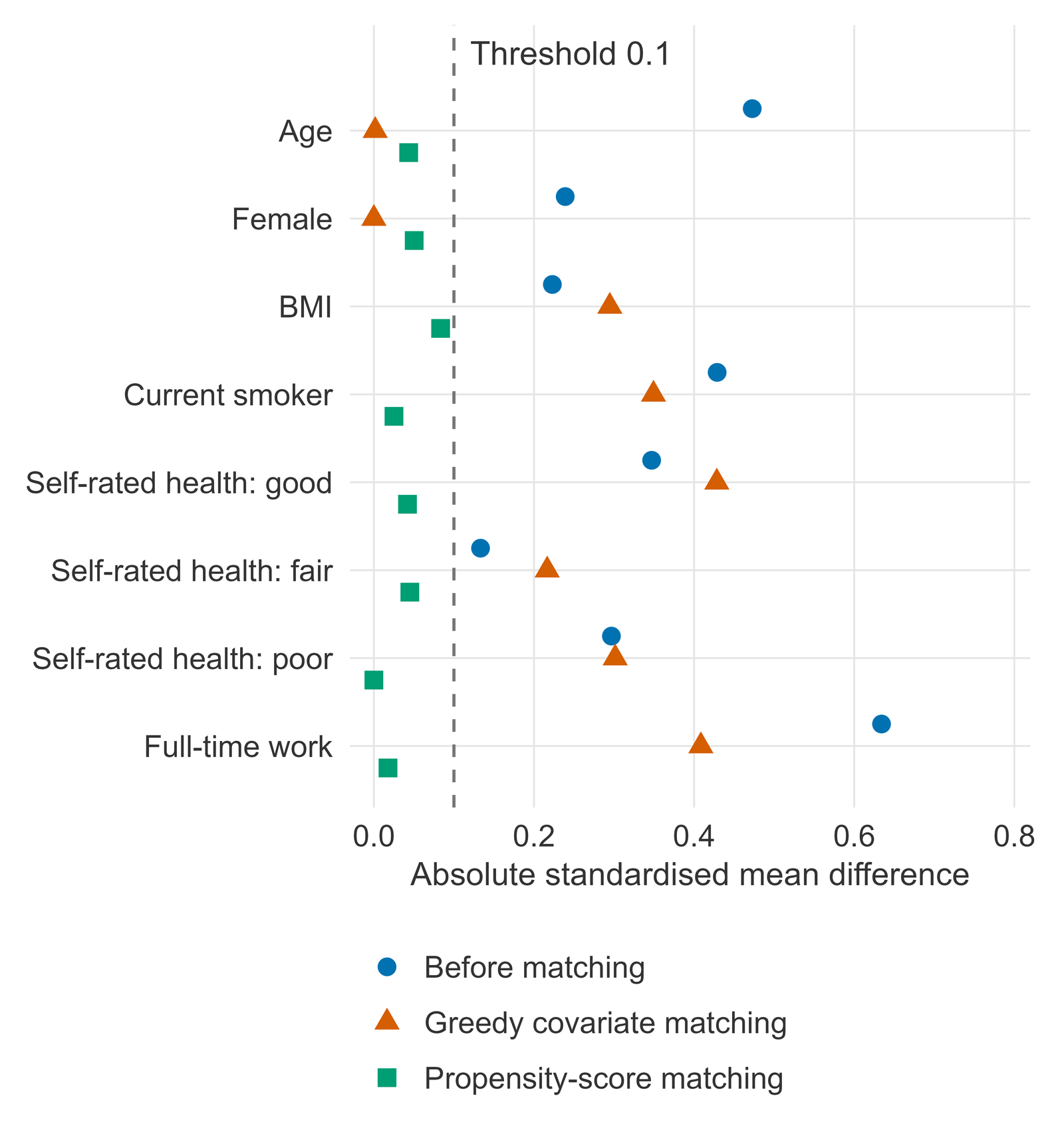
How to read it: each row is one covariate and each point is one sample. A point left of the dashed line is balanced by the 0.1 rule. Read along a row to see what each method did to that covariate: for full-time work, the point moves from 0.63 before matching to 0.41 after greedy matching and 0.02 after propensity-score matching.วิธีอ่าน: แต่ละแถวคือตัวแปรร่วมหนึ่งตัว และแต่ละจุดคือตัวอย่างหนึ่งชุด จุดที่อยู่ทางซ้ายของเส้นประถือว่าสมดุลตามเกณฑ์ 0.1 อ่านไล่ไปตามแถวเพื่อดูว่าแต่ละวิธีเปลี่ยนตัวแปรร่วมนั้นอย่างไร เช่น การทำงานเต็มเวลา จุดเลื่อนจาก 0.63 ก่อนการจับคู่ เป็น 0.41 หลังการจับคู่แบบ greedy และ 0.02 หลังการจับคู่ด้วย propensity score
The outcome in the matched groupsผลลัพธ์ในกลุ่มที่จับคู่แล้ว
Each comparison fits the same linear probability model, active = intercept + risk difference × joined, so the coefficient of joined is the risk difference. In the matched samples its 95% confidence interval uses standard errors clustered on the matched pair (sandwich estimator), because the two people in a pair were chosen to be alike and their outcomes are not independent; for one-to-one pairs this is the Wald interval for paired proportions built from the discordant pairs. These standard errors treat the estimated propensity score as known. The crude row uses a heteroscedasticity-robust standard error, the usual Wald interval for two independent proportions. Because the data are simulated, each person's chance of being active with and without the programme is known, so the table also gives the true risk difference averaged over the joined people in the same row.การเปรียบเทียบทุกแบบใช้แบบจำลองความน่าจะเป็นเชิงเส้น (linear probability model) แบบเดียวกัน คือ การมีกิจกรรมทางกาย = ค่าคงที่ + ผลต่างความเสี่ยง × การเข้าร่วม สัมประสิทธิ์ของการเข้าร่วมจึงเป็นผลต่างความเสี่ยงโดยตรง ในตัวอย่างที่จับคู่ ช่วงความเชื่อมั่น 95% คำนวณจากค่าความคลาดเคลื่อนมาตรฐานแบบคลัสเตอร์ตามคู่ (sandwich estimator) เพราะคนสองคนในคู่เดียวกันถูกเลือกให้มีลักษณะคล้ายกัน ผลลัพธ์ของทั้งคู่จึงไม่เป็นอิสระต่อกัน สำหรับการจับคู่แบบหนึ่งต่อหนึ่ง ช่วงนี้เท่ากับช่วงความเชื่อมั่นแบบ Wald ของสัดส่วนที่จับคู่ (paired proportions) ซึ่งคำนวณจากคู่ที่ผลลัพธ์ไม่ตรงกัน (discordant pairs) ค่าความคลาดเคลื่อนมาตรฐานนี้ถือว่า propensity score ที่ประมาณได้เป็นค่าที่ทราบแน่นอน ส่วนแถว crude ใช้ค่าความคลาดเคลื่อนมาตรฐานแบบ heteroscedasticity-robust ซึ่งเท่ากับช่วงความเชื่อมั่นแบบ Wald ของสองสัดส่วนที่เป็นอิสระต่อกัน เนื่องจากเป็นข้อมูลจำลอง จึงทราบโอกาสที่แต่ละคนจะมีกิจกรรมทางกายถึงเป้าหมายทั้งเมื่อเข้าร่วมและไม่เข้าร่วม ตารางจึงแสดงผลต่างความเสี่ยงที่แท้จริงซึ่งเฉลี่ยจากผู้เข้าร่วมในแถวเดียวกันไว้ด้วย
| Comparison | Joined, n | Did not join, n | Physically active a year later | Joined minus did not join, percentage points | ||
|---|---|---|---|---|---|---|
| Active, joined | Active, did not join | Risk difference (95% CI) | True risk difference | |||
| Crude: everybody, unmatched | 268 | 732 | 43.3% | 22.8% | 20.5 (13.8 to 27.1) | 12.5 |
| Greedy covariate matching | 261 | 261 | 43.7% | 20.7% | 23.0 (15.2 to 30.7) | 12.4 |
| Propensity-score matching | 242 | 242 | 41.3% | 31.0% | 10.3 (1.9 to 18.8) | 12.3 |
- Risk difference: joined minus did not join, in percentage points, from a linear probability model. Crude row: Wald 95% CI with a heteroscedasticity-robust standard error. Matched rows: Wald 95% CI with standard errors clustered on the matched pair (sandwich, no small-sample correction), equal to the Wald interval for paired proportions; the propensity score is treated as known.ผลต่างความเสี่ยง คือ ผู้เข้าร่วมลบผู้ที่ไม่ได้เข้าร่วม หน่วยเป็นจุดร้อยละ จากแบบจำลองความน่าจะเป็นเชิงเส้น แถว crude: ช่วงความเชื่อมั่น 95% แบบ Wald จากค่าความคลาดเคลื่อนมาตรฐานแบบ heteroscedasticity-robust แถวที่จับคู่: ช่วงความเชื่อมั่น 95% แบบ Wald จากค่าความคลาดเคลื่อนมาตรฐานแบบคลัสเตอร์ตามคู่ (sandwich ไม่มีการปรับสำหรับตัวอย่างขนาดเล็ก) ซึ่งเท่ากับช่วงแบบ Wald ของสัดส่วนที่จับคู่ และถือว่า propensity score เป็นค่าที่ทราบแน่นอน
- True risk difference: the mean, over the joined people in that row, of each person's simulated chance of being active if they joined minus their chance if they did not. It is known only because the data are simulated.ผลต่างความเสี่ยงที่แท้จริง คือ ค่าเฉลี่ยของผลต่างระหว่างโอกาสจำลองที่จะมีกิจกรรมทางกายถึงเป้าหมายเมื่อเข้าร่วมกับเมื่อไม่เข้าร่วม ของผู้เข้าร่วมแต่ละคนในแถวนั้น ค่านี้ทราบได้เพราะเป็นข้อมูลจำลองเท่านั้น
- CI, confidence interval.CI คือช่วงความเชื่อมั่น
How to read it: compare each estimate with the truth in the same row. The crude difference, 20.5 percentage points (95% CI 13.8 to 27.1), is larger than the true effect in all who joined, 12.5, because the people who joined were more likely to be active even without the programme. Greedy matching gave 23.0 (15.2 to 30.7); its interval lies above the true 12.4 for the joined people it matched, because the covariates it did not match on are still imbalanced. Propensity-score matching gave 10.3 (1.9 to 18.8), an interval that includes the true 12.3 for the joined people it matched. That true value is close to the 12.5 for everyone who joined, but it is a different group: the estimate describes the matched joined people only.วิธีอ่าน: เทียบค่าประมาณแต่ละค่ากับผลที่แท้จริงในแถวเดียวกัน ผลต่างแบบหยาบเท่ากับ 20.5 จุดร้อยละ (ช่วงความเชื่อมั่น 95% 13.8 ถึง 27.1) สูงกว่าผลที่แท้จริงในผู้เข้าร่วมทั้งหมดซึ่งเท่ากับ 12.5 เพราะผู้ที่เข้าร่วมมีโอกาสมีกิจกรรมทางกายถึงเป้าหมายสูงกว่าอยู่แล้วแม้ไม่มีโครงการ การจับคู่แบบ greedy ได้ 23.0 (15.2 ถึง 30.7) ช่วงนี้อยู่สูงกว่าผลที่แท้จริงของผู้เข้าร่วมที่ได้รับการจับคู่ด้วยวิธีนี้ซึ่งเท่ากับ 12.4 เพราะตัวแปรร่วมที่ไม่ได้ใช้จับคู่ยังไม่สมดุล การจับคู่ด้วย propensity score ได้ 10.3 (1.9 ถึง 18.8) ซึ่งครอบคลุมผลที่แท้จริงของผู้เข้าร่วมที่ได้รับการจับคู่ด้วยวิธีนี้คือ 12.3 ค่าที่แท้จริงนี้ใกล้เคียงกับ 12.5 ของผู้เข้าร่วมทั้งหมด แต่เป็นคนละกลุ่มกัน ค่าประมาณนี้จึงอธิบายเฉพาะผู้เข้าร่วมที่ได้รับการจับคู่เท่านั้น
What matching does and does not do. Matching balances only the covariates that were measured and used; a confounder that was not measured, such as motivation to exercise, can stay imbalanced, and no balance table can show it. The estimate applies to the matched people who joined (the ATT), not to everyone screened. When people who joined are left unmatched, the result is about a narrower group, so the number left unmatched, and how they differ, should always be reported. Balance is judged by standardised differences, not by P values.สิ่งที่การจับคู่ทำได้และทำไม่ได้ การจับคู่ทำให้สมดุลได้เฉพาะตัวแปรร่วมที่วัดและนำมาใช้เท่านั้น ตัวแปรกวน (confounder) ที่ไม่ได้วัด เช่น แรงจูงใจในการออกกำลังกาย อาจยังไม่สมดุล และไม่มีตารางความสมดุลใดแสดงให้เห็นได้ ค่าประมาณที่ได้ใช้กับผู้เข้าร่วมที่ได้รับการจับคู่ (ATT) ไม่ใช่กับทุกคนที่มารับการตรวจคัดกรอง เมื่อมีผู้เข้าร่วมที่ไม่ได้รับการจับคู่ ผลที่ได้จะเป็นของกลุ่มที่แคบลง จึงควรรายงานจำนวนผู้ที่ไม่ได้รับการจับคู่และลักษณะที่แตกต่างของคนกลุ่มนี้เสมอ และความสมดุลตัดสินจาก standardised difference ไม่ใช่จากค่า P
Methods paragraph for a manuscriptย่อหน้าวิธีการทางสถิติสำหรับต้นฉบับบทความ
Statistical analysis. To estimate the effect of joining the programme among those who joined (the average treatment effect on the treated, restricted to the joined people who could be matched), people who joined were matched one-to-one without replacement to people who did not join, by two methods: greedy nearest-neighbour matching on covariates, exact on sex and nearest on age within 2 years; and greedy nearest-neighbour matching on the logit of a propensity score estimated by logistic regression of joining on age, sex, body-mass index, current smoking, self-rated health (good, fair, poor) and full-time work, with a caliper of 0.2 pooled standard deviations of the logit of the propensity score, matching from the highest score down. Covariate balance was assessed with standardised mean differences, with the pooled standard deviation before matching as the denominator; an absolute value below 0.1 was taken to indicate balance. The outcome was compared with a linear probability model giving the risk difference, with a Wald 95% confidence interval from standard errors clustered on the matched pair, treating the propensity score as known. The number of people who joined but were not matched is reported for each method, with the characteristics of those the propensity-score match left out. Analyses were done in R version 4.6.1 with MatchIt 4.7.2, cobalt 5.0.0 and sandwich 3.1.1.การวิเคราะห์ทางสถิติ เพื่อประมาณผลของการเข้าร่วมโครงการในกลุ่มผู้ที่เข้าร่วม (average treatment effect on the treated เฉพาะผู้เข้าร่วมที่สามารถจับคู่ได้) ผู้เข้าร่วมได้รับการจับคู่กับผู้ที่ไม่ได้เข้าร่วมแบบหนึ่งต่อหนึ่งโดยไม่ใช้ซ้ำ ด้วยสองวิธี ได้แก่ การจับคู่แบบ greedy nearest-neighbour บนตัวแปรร่วม โดยให้เพศตรงกันและอายุใกล้ที่สุดภายใน 2 ปี และการจับคู่แบบ greedy nearest-neighbour บนค่า logit ของ propensity score ที่ประมาณจากการถดถอยลอจิสติกที่มีการเข้าร่วมเป็นตัวแปรตาม และมีอายุ เพศ ดัชนีมวลกาย การสูบบุหรี่ในปัจจุบัน สุขภาพที่ประเมินด้วยตนเอง (ดี พอใช้ ไม่ดี) และการทำงานเต็มเวลาเป็นตัวแปรอิสระ โดยใช้ caliper เท่ากับ 0.2 เท่าของส่วนเบี่ยงเบนมาตรฐานรวมของ logit ของ propensity score และจับคู่จากคะแนนสูงสุดลงมา ประเมินความสมดุลของตัวแปรร่วมด้วย standardised mean difference โดยใช้ส่วนเบี่ยงเบนมาตรฐานรวมก่อนการจับคู่เป็นตัวหาร และถือว่าค่าสัมบูรณ์ที่ต่ำกว่า 0.1 แสดงถึงความสมดุล เปรียบเทียบผลลัพธ์ด้วยแบบจำลองความน่าจะเป็นเชิงเส้นซึ่งให้ผลต่างความเสี่ยง พร้อมช่วงความเชื่อมั่น 95% แบบ Wald จากค่าความคลาดเคลื่อนมาตรฐานแบบคลัสเตอร์ตามคู่ โดยถือว่า propensity score เป็นค่าที่ทราบแน่นอน และรายงานจำนวนผู้เข้าร่วมที่ไม่ได้รับการจับคู่ของแต่ละวิธี พร้อมลักษณะของผู้เข้าร่วมที่การจับคู่ด้วย propensity score หาคู่ให้ไม่ได้ วิเคราะห์ด้วยโปรแกรม R เวอร์ชัน 4.6.1 ร่วมกับแพ็กเกจ MatchIt 4.7.2 cobalt 5.0.0 และ sandwich 3.1.1
What this sample does not show: no sensitivity analysis for unmeasured confounding, no covariate adjustment after matching, no comparison with weighting or a doubly robust estimator, no balance measure other than the standardised mean difference, such as variance ratios, and no plot of propensity-score overlap (common support). Whether the programme works, for whom, and what to do next is for the research team to interpret.สิ่งที่ตัวอย่างนี้ไม่ได้แสดง: ไม่มีการวิเคราะห์ความไวต่อตัวแปรกวนที่ไม่ได้วัด (sensitivity analysis for unmeasured confounding) ไม่มีการปรับตัวแปรร่วมเพิ่มเติมหลังการจับคู่ ไม่มีการเปรียบเทียบกับวิธีถ่วงน้ำหนัก (weighting) หรือตัวประมาณแบบ doubly robust ไม่มีตัวชี้วัดความสมดุลอื่นนอกจาก standardised mean difference เช่น variance ratio และไม่มีแผนภาพแสดงการซ้อนทับของ propensity score ระหว่างสองกลุ่ม (common support) การตัดสินว่าโครงการได้ผลหรือไม่ ได้ผลกับใคร และควรทำอะไรต่อ เป็นหน้าที่ของทีมวิจัยในการแปลผล
What you send and do yourselfสิ่งที่คุณต้องส่งและทำเอง
- The exposure, the outcome and the variables to match on, with your reasons.ปัจจัยที่ศึกษา ผลลัพธ์ และตัวแปรที่ต้องการใช้จับคู่ พร้อมเหตุผล
- A de-identified dataset with its codebook: no names, ID numbers, addresses or anything else that identifies a person.ชุดข้อมูลที่ตัดข้อมูลระบุตัวตนออกแล้ว พร้อมคู่มือรหัสตัวแปร (codebook) โดยไม่มีชื่อ เลขประจำตัว ที่อยู่ หรือข้อมูลอื่นที่ระบุตัวบุคคลได้
- You interpret the results and write your own article, and acknowledge the statistical help in the way your journal asks.คุณเป็นผู้แปลผลและเขียนบทความของคุณเอง และระบุความช่วยเหลือด้านสถิติตามรูปแบบที่วารสารกำหนด
Limitsขอบเขตและข้อจำกัด
- Statistical analysis and advice only: the research question, the data, the interpretation and the writing stay yours.บริการนี้เป็นงานวิเคราะห์และให้คำแนะนำทางสถิติเท่านั้น คำถามวิจัย ข้อมูล การแปลผล และการเขียน เป็นของคุณทั้งหมด
- Matching balances only the variables that were measured; it cannot remove confounding by anything unmeasured.การจับคู่ทำให้สมดุลได้เฉพาะตัวแปรที่วัดไว้ ไม่สามารถขจัดอิทธิพลของตัวแปรกวนที่ไม่ได้วัด
- Propensity-score weighting or stratification and other causal-inference analyses are not offered at present.ขณะนี้ยังไม่รับงานถ่วงน้ำหนักหรือแบ่งชั้นด้วยคะแนนแนวโน้ม (propensity score) และงานวิเคราะห์เชิงสาเหตุรูปแบบอื่น
- Not for a thesis, an independent study or other work submitted for a degree; for those, I offer consultation only.ไม่รับทำงานที่จะนำไปใช้เพื่อสำเร็จการศึกษา เช่น วิทยานิพนธ์ การค้นคว้าอิสระ หรือผลงานอื่นที่ยื่นเพื่อรับปริญญา งานลักษณะนี้รับเฉพาะการให้คำปรึกษา
- Authorship is not sold and is not a condition of the service.การมีชื่อเป็นผู้นิพนธ์ไม่ใช่สิ่งที่ซื้อขายได้ และไม่ใช่เงื่อนไขในการรับงาน
Request this serviceขอใช้บริการนี้
Every request is reviewed first. I may accept or decline it. The timeline is agreed per project after review.ผมพิจารณาคำขอทุกงานก่อน และอาจรับหรือปฏิเสธงาน ระยะเวลาของแต่ละงานตกลงกันหลังพิจารณาคำขอแล้ว
Member prices apply only to orders that start on uniqcret.com; if you found me on Fastwork or your enquiry began there, please order on Fastwork at the Fastwork price.ราคาสมาชิกใช้กับงานที่เริ่มต้นบน uniqcret.com เท่านั้น หากคุณรู้จักผมจาก Fastwork หรือเริ่มสอบถามบน Fastwork กรุณาสั่งงานบน Fastwork ในราคาของ Fastwork