Understanding ROC Curve Geometry: How AUC Visualizes Outcome Separation

Mayta
Oct 5
3 min read

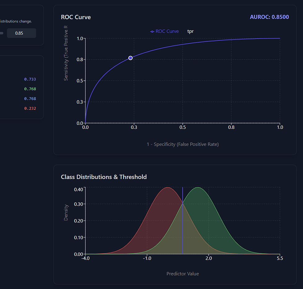
Web Application to visualize how ROC Influential Divide the ability outcome Y.

🎯 ROC as the Geometry of Outcome Separation

When you measure a continuous test result or prediction score ( X ), it generates two overlapping distributions:

f1(x) : distribution of scores among those with the outcome (Y = 1)
f0(x) : distribution of scores among those without the outcome (Y = 0)

The ROC curve and its Area under the Curve (AUC) summarize how separable these two distributions are.

1️⃣ When AUC = 0.5 → “Complete Overlap”

If ROC = 0.5, the two distributions perfectly overlap — meaning the test or model offers no discriminative information. Mathematically: f1(x) = f0(x)

In this case, the probability that a randomly selected patient with the outcome (Y = 1) has a higher test value than a patient without (Y = 0) is 0.5 — purely random guessing.Visually, both curves form a single bell-shaped distribution, indistinguishable from each other.

Clinical meaning: The lab value (test result) behaves identically in diseased and non-diseased groups — no diagnostic or predictive signal at all.

2️⃣ When AUC = 1.0 → “Perfect Separation”

If ROC = 1.0, the two distributions are completely separated — there is zero overlap. That is: f1(x)∩f0(x)=∅

The test perfectly distinguishes between outcome states; every Y = 1 observation scores higher than every Y = 0.Graphically, this looks like two distinct normal distributions, entirely split apart — one to the left (non-diseased), one to the right (diseased).

Clinical meaning: The test or model assigns non-overlapping scores; a single threshold can classify all cases correctly with 100 % sensitivity and 100 % specificity.

3️⃣ Between the Extremes (0.5 < AUC < 1.0)

Most real-world ROC values fall between 0.6 – 0.9.This means the two distributions partially overlap:

The degree of overlap decreases as AUC increases.
The distance between the means of f1(x) and f0(x) determines the AUC value.

If both f1(x) and f0(x) are normal with equal variance σ^2 , the link between the mean separation (d′) and the AUC is:

AUC = Φ*(d'*2^(1/2))

where ( Φ ) is the cumulative distribution function of the standard normal.Thus:

( d' = 0 ) → AUC = 0.5 (complete overlap)
( d' ≈ 2.83 ) → AUC ≈ 0.99 (near-perfect split)

This is the mathematical bridge between the signal-detection theory of ROC and the normal distribution geometry you described.

4️⃣ Visual Analogy (Narrative)

AUC	Distributions of Predicted Score (X) by Outcome (Y)	Description
0.5	🎯 One merged bell curve	No discrimination
0.7	🎯🎯 Two overlapping bell curves	Acceptable discrimination
0.9	🎯 🎯 Two mostly separated curves	Excellent discrimination
1.0	🎯 🎯 Perfect split	Ideal discrimination

5️⃣ Conceptual Integration (Clinical Research View)

ROC quantifies how Y is divided by X.
Higher AUC means Y’s two conditional distributions become more separated, allowing clinicians to apply a single threshold that meaningfully distinguishes patient outcomes.
However, this does not imply perfect calibration — the predicted probabilities can still be systematically too high or too low, even with a high ROC.

✅ Key Takeaways

AUC = 0.5 → identical distributions (no separation).
AUC = 1.0 → non-overlapping distributions (perfect separation).
Intermediate AUC values reflect partial overlap — quantified by ( d' ) or mean difference.
ROC = geometry of outcome division — it visualizes how prediction reshapes Y.